Topics
The alert fired on a Tuesday, six weeks after the regression shipped. The post-mortem asked why nobody noticed sooner, and the answer was in the monitor's own design: a three-sigma rule on a daily metric takes about six weeks to catch a shift of that size. Nothing failed. The monitor did what it was built to do, at the speed it was built to do it, and nobody had ever computed that speed.
A monitor is described by two numbers, not one. How long it runs before crying wolf, and how long it takes to notice a real change. Tightening the threshold improves the second and ruins the first. Choosing a better chart improves both.
The Threshold Sets the False Alarm Interval
For a fixed threshold applied every day to an independent metric, the days until a false alarm follow a geometric distribution, so the average is one over the daily signal probability.
1
2
3
4
5
6
7
8
9
10
11
12
13
14
15
16
17
18
19
20
21
22
23
24
25
26
27
28
29
30
31
32
33
34
35
36
37
38
39
40
41
42
43
44
45
46
47
48
49
50
51
52
53
54
55
56
import numpy as np
from scipy import stats

RNG = np.random.default_rng(47)
REPS = 20000
MAX_DAYS = 4000


def shewhart(x, limit):
    return np.abs(x) > limit


def ewma_signal(x, lam, limit):
    """Exponentially weighted average against its own standard deviation."""
    z = np.zeros_like(x)
    acc = 0.0
    for i, v in enumerate(x):
        acc = lam * v + (1 - lam) * acc
        z[i] = acc
    sd = np.sqrt(lam / (2 - lam) * (1 - (1 - lam) ** (2 * (np.arange(len(x)) + 1))))
    return np.abs(z) > limit * sd


def cusum_signal(x, k, h):
    """Two one-sided cumulative sums of the excess over k."""
    hi = lo = 0.0
    out = np.zeros(len(x), bool)
    for i, v in enumerate(x):
        hi = max(0.0, hi + v - k)
        lo = max(0.0, lo - v - k)
        out[i] = (hi > h) or (lo > h)
    return out


def run_length(shift, kind, param, reps=REPS, rng=RNG):
    """Days until the first signal, with the shift present from day one."""
    lengths = np.empty(reps)
    for r in range(reps):
        x = rng.normal(shift, 1.0, MAX_DAYS)
        if kind == "shewhart":
            sig = shewhart(x, param)
        elif kind == "ewma":
            sig = ewma_signal(x, 0.2, param)
        else:
            sig = cusum_signal(x, 0.5, param)
        idx = np.argmax(sig)
        lengths[r] = idx + 1 if sig[idx] else MAX_DAYS
    return lengths


p = 2 * (1 - stats.norm.cdf(3))
print(f"chance of a signal on any day: {p:.4%}")
print(f"average days between false alarms: {1 / p:6.0f}")
print(f"median days: {np.log(0.5) / np.log(1 - p):6.0f}")
for q in (0.10, 0.25, 0.50):
    print(f"  {q:.0%} of false alarms arrive within {np.log(1 - q) / np.log(1 - p):5.0f} days")
| Quantity | Value |
|---|---|
| Chance of a signal on any day | 0.2700% |
| Average days between false alarms | 370 |
| Median days | 256 |
| A tenth of false alarms arrive within | 39 days |
| A quarter within | 106 days |
| Half within | 256 days |
The famous 370 is an average over a distribution with a long tail, and the median is 256. More usefully, one false alarm in ten arrives inside the first 39 days. A team that installs a three-sigma monitor and sees it fire in the second month has not found a bug in the monitor; they have seen the tenth percentile.
Same False Alarm Rate, Different Speed
The Shewhart rule looks at today only. A cumulative sum accumulates small excesses until they add up, and an exponentially weighted average blends today with the recent past. Both notice small persistent shifts sooner, and the comparison is only meaningful once all three are tuned to the same false alarm rate.
1
2
3
4
5
6
7
8
9
10
11
12
13
14
15
16
17
18
19
20
21
22
23
24
# Calibrate EWMA and CUSUM to an in-control run length near the Shewhart 370.
LIMITS = {}
for kind, lo, hi in (("ewma", 2.0, 3.6), ("cusum", 2.0, 8.0)):
    for _ in range(18):
        mid = (lo + hi) / 2
        arl0 = run_length(0.0, kind, mid, reps=1200,
                          rng=np.random.default_rng(5)).mean()
        if arl0 < 370:
            lo = mid
        else:
            hi = mid
    LIMITS[kind] = (lo + hi) / 2
LIMITS["shewhart"] = 3.0
print(f"limits: Shewhart {LIMITS['shewhart']:.2f} sigma, "
      f"EWMA {LIMITS['ewma']:.2f}, CUSUM h = {LIMITS['cusum']:.2f}")

print(f"{'shift':>8} {'Shewhart':>22} {'EWMA':>22} {'CUSUM':>22}")
for shift in (0.0, 0.5, 1.0, 1.5, 2.0, 3.0):
    row = []
    for kind in ("shewhart", "ewma", "cusum"):
        L = run_length(shift, kind, LIMITS[kind], reps=4000,
                       rng=np.random.default_rng(9))
        row.append(f"{L.mean():7.1f} (median {np.median(L):5.0f})")
    print(f"{shift:8.1f} " + " ".join(f"{c:>22}" for c in row))
The calibration lands on an exponentially weighted limit of 2.86 and a cumulative sum limit of 4.72, both giving roughly the same in-control run length as a three-sigma rule.
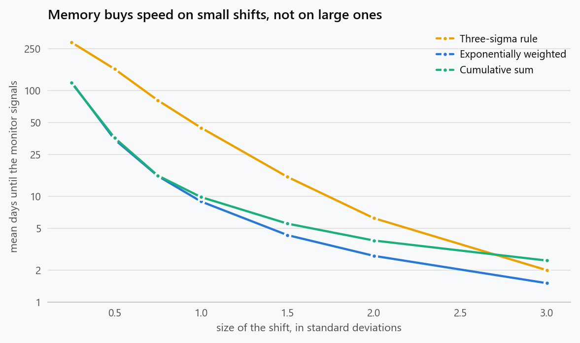
| Shift, in standard deviations | Shewhart, mean days (median) | Exponentially weighted, mean (median) | Cumulative sum, mean (median) |
|---|---|---|---|
| 0.0 | 378.4 (263) | 359.2 (245) | 347.5 (246) |
| 0.5 | 157.0 (110) | 35.5 (26) | 34.7 (26) |
| 1.0 | 44.0 (31) | 8.8 (7) | 9.9 (9) |
| 1.5 | 15.1 (11) | 4.3 (4) | 5.5 (5) |
| 2.0 | 6.4 (5) | 2.7 (2) | 3.8 (4) |
| 3.0 | 2.0 (1) | 1.5 (1) | 2.5 (2) |
The first row confirms the three charts are comparable: all three run around 350 to 380 days between false alarms. Every other row is the argument for changing chart. A half-sigma shift takes the three-sigma rule 157 days on average and the other two about 35. A one-sigma shift takes 44 days against nine. The advantage narrows as the shift grows and vanishes above two sigma, where any rule catches it within days.
That pattern has a simple explanation. A large shift shows up in a single observation, which is exactly what the Shewhart rule is good at. A small shift never produces an extreme day; it produces a long run of slightly high days, which only a chart with memory can see.
The Average Is the Wrong Summary
Detection delay is as skewed as the false alarm interval, so an average conceals both the lucky cases and the ones that matter.
1
2
3
4
5
L = run_length(1.0, "shewhart", 3.0, reps=8000, rng=np.random.default_rng(11))
print(f"one-sigma shift on a three-sigma rule: mean {L.mean():.1f} days, "
      f"median {np.median(L):.0f}")
for q in (0.10, 0.25, 0.50, 0.75, 0.90):
    print(f"  {q:.0%} of shifts are caught within {np.quantile(L, q):5.0f} days")
| Share of shifts caught | Within |
|---|---|
| 10% | 5 days |
| 25% | 13 days |
| 50% | 31 days |
| 75% | 61 days |
| 90% | 99 days |
Mean 44 days, median 31, and one time in ten the shift runs for more than three months before the monitor says anything. When the question is "how long could a regression hide", the ninetieth percentile is the number that belongs in the design document, not the mean.
Correlated Days Destroy the Calibration
Everything above assumes today's value is independent of yesterday's. Operational metrics rarely are: traffic mix, weather, campaigns and backlogs all persist. The damage is not subtle, and it comes through the way limits are usually estimated, from the average moving range between consecutive days.
1
2
3
4
5
6
7
8
9
10
11
12
13
14
15
16
17
for rho in (0.0, 0.3, 0.6, 0.8):
    ratios, signals = [], []
    rng = np.random.default_rng(13)
    for _ in range(2000):
        eps = rng.normal(0, np.sqrt(1 - rho ** 2), 500)
        x = np.zeros(500)
        for i in range(1, 500):
            x[i] = rho * x[i - 1] + eps[i]
        # The individuals chart estimates sigma from the average moving range.
        base = x[:200]
        sigma_hat = np.abs(np.diff(base)).mean() / 1.128
        ratios.append(sigma_hat)
        signals.append((np.abs(x[200:]) > 3 * sigma_hat).sum())
    daily = np.mean(signals) / 300
    print(f"day-to-day correlation {rho:3.1f}: estimated sigma {np.mean(ratios):5.2f} "
          f"against a true 1.00, false signals {np.mean(signals):6.1f} per 300 days, "
          f"one every {1 / daily if daily else float('inf'):7.1f} days")
| Day-to-day correlation | Estimated standard deviation | False signals per 300 days | One false alarm every |
|---|---|---|---|
| 0.0 | 1.00 | 1.0 | 307 days |
| 0.3 | 0.84 | 4.0 | 76 days |
| 0.6 | 0.63 | 17.7 | 17 days |
| 0.8 | 0.45 | 54.2 | 5.5 days |
The estimated standard deviation follows $\sqrt{1-\rho}$ almost exactly, because the moving range measures the variability between adjacent days and adjacent days are similar when the series drifts. At a correlation of 0.8 the chart believes the metric is half as variable as it is, sets its limits accordingly, and fires every five or six days.
This is the most common reason monitoring gets switched off. The chart is not badly designed and the metric is not broken; the limits were estimated with a method that assumes independence, applied to a metric that has none. The fix is to estimate the standard deviation from the long-run spread rather than from consecutive differences, to monitor a residual after removing the predictable part, or to aggregate to a period over which the correlation has died away.
Choosing the Two Numbers
The design conversation is short once the numbers are on the table. Decide how often a false alarm is tolerable, which in most teams is set by how much attention an alert consumes. Decide the smallest shift worth catching and how quickly. Then pick the chart that meets both, which for small persistent shifts is almost never a single-point threshold.
One caution about tightening. Moving a Shewhart limit from three sigma to two cuts the mean detection delay for a one-sigma shift from 44 days to about 6, and cuts the false alarm interval from 370 days to 22. That is usually the wrong trade, and it is the trade teams make by instinct when an incident is fresh. Switching to a chart with memory buys the same detection speed while keeping the alarm interval.
What to Do
- Write both numbers into the monitor's definition: the expected days between false alarms, and the expected days to catch the smallest shift that matters.
- Report the ninetieth percentile of the detection delay, not the average. That is the exposure window an incident review will ask about.
- Use a cumulative sum or exponentially weighted chart for small persistent shifts. At the same false alarm rate they are four to five times faster at shifts of half to one sigma.
- Keep a single-point rule alongside them for large jumps, where it is the fastest and simplest thing available.
- Estimate limits from the long-run spread, never from consecutive differences, unless the metric is genuinely independent day to day.
- Measure the autocorrelation of every monitored metric before setting limits. Above about 0.3 the nominal alarm interval is fiction.
The figure generator in the blog-reproducibility repository reproduces this article's figure; run it with --dry-run to print the numbers behind the figure without writing an image.
References
- Page, E. S. (1954). Continuous inspection schemes. Biometrika, 41(1-2), 100-115.
- Roberts, S. W. (1959). Control chart tests based on geometric moving averages. Technometrics, 1(3), 239-250.
- Lucas, J. M., & Saccucci, M. S. (1990). Exponentially weighted moving average control schemes: properties and enhancements. Technometrics, 32(1), 1-12.
- Montgomery, D. C. (2019). Introduction to Statistical Quality Control (8th ed.). Wiley.
- Alwan, L. C., & Roberts, H. V. (1988). Time-series modeling for statistical process control. Journal of Business and Economic Statistics, 6(1), 87-95.
- Woodall, W. H., & Montgomery, D. C. (2014). Some current directions in the theory and application of statistical process monitoring. Journal of Quality Technology, 46(1), 78-94.
Embed interactive plots, widgets, and demos using <figure>, <iframe>, or <div class="interactive-embed"> containers. Ensure each embed includes descriptive captions for accessibility.
How to cite
Use the quick export buttons to save citations for reference managers or copy the formatted text directly.
Diogo Ribeiro (2025). Run Length: How Long Your Monitor Takes to Notice. Faculty of Media Arts and Design, Technical University of Porto. https://diogoribeiro7.github.io/statistics/run_length_how_long_a_monitor_takes/.


