Topics
The feature distributions look unchanged. The model's confidence is unchanged. Its positive prediction rate is unchanged. The monitoring dashboard is green.
What does that establish about accuracy?
Without outcomes or additional assumptions, very little. We can construct two environments with exactly the same quantities available to the dashboard and sharply different accuracy. This is an identification problem, rather than a shortage of clever drift statistics.
Unlabelled monitoring remains useful. It can reveal broken schemas, changes in traffic, missing features, unexpected scores, and violations of operational constraints. The important boundary is between observing those changes and claiming to know how often the predictions are right.
Write down what the monitor observes
For a fixed classifier $h$, let $X$ be its input, $Y$ the eventual outcome, $S=f(X)$ its score, and $\widehat Y=h(X)$ its prediction. Before outcomes arrive, the monitor observes samples of $(X,S,\widehat Y)$ and any available operational measurements.
For a loss function $L$, production risk is
Unlabelled inputs supply information about $p_t(x)$. Predictions and scores are functions of those inputs and the fixed model. They do not, by themselves, identify the current relationship $p_t(y\mid x)$.
This distinction persists even with infinitely many unlabelled observations. More data can estimate the observable distribution more precisely while leaving the missing relationship unresolved.
Two indistinguishable environments
Let $X$ take values zero and one with equal probability. The model predicts $\widehat Y=X$ and reports the probability score
Consider two possible joint distributions:
| $X$ | $Y$ | Reference environment | Hidden reversal |
|---|---|---|---|
| 0 | 0 | 0.45 | 0.05 |
| 0 | 1 | 0.05 | 0.45 |
| 1 | 0 | 0.05 | 0.45 |
| 1 | 1 | 0.45 | 0.05 |
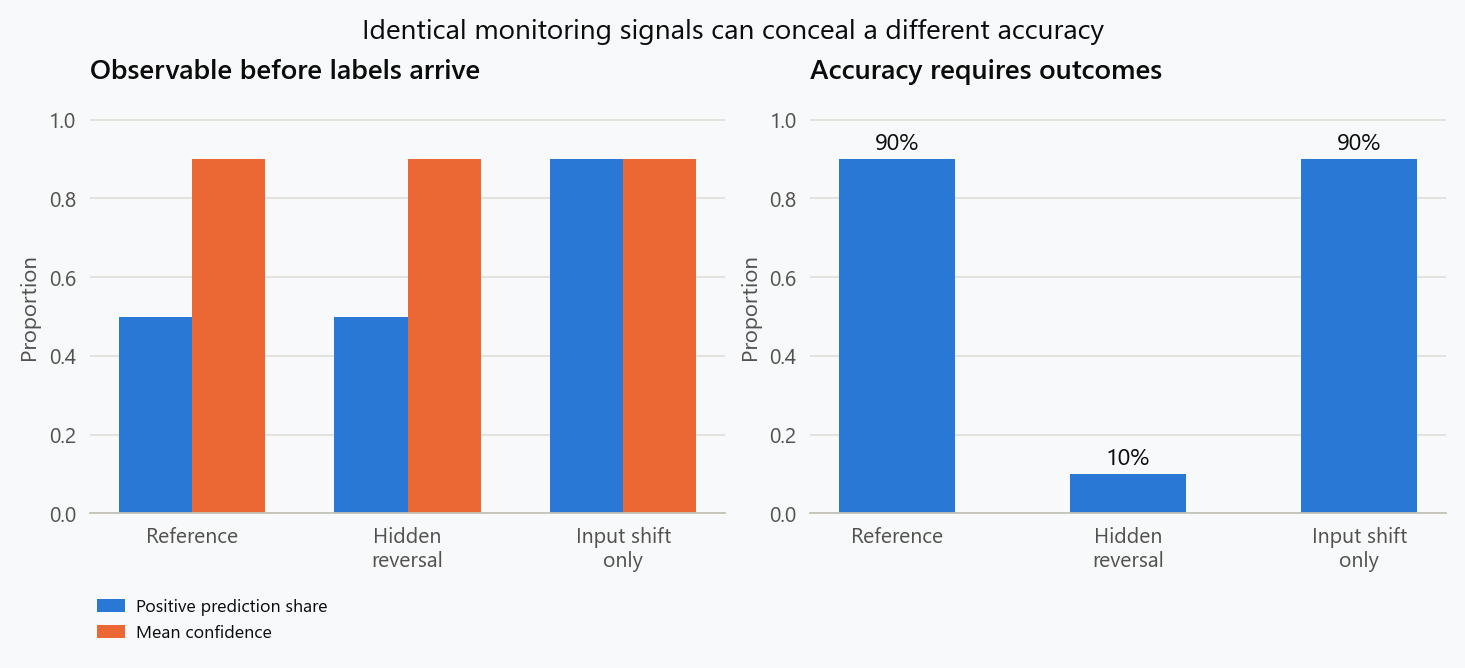
Both environments have $P(X=1)=0.5$. Therefore both have the same prediction distribution, the same score distribution, and mean reported confidence $E[\max(S,1-S)]=0.9$. Even their outcome prevalences are identical: $P(Y=1)=0.5$.
In the reference environment, the classifier is correct on the two diagonal cells, whose probabilities sum to 0.9. In the reversal environment, those cells sum to 0.1.
The accuracy changes from 90 percent to 10 percent while every unlabelled quantity in this example stays fixed. Knowing only the marginal outcome prevalence would not resolve the ambiguity either.
The scores are calibrated in the reference environment: among observations with score 0.9, the positive outcome probability is 0.9. They are badly miscalibrated after the reversal. Calibration requires outcomes to assess, so an unchanged score histogram cannot establish that calibration transferred.
There is no test on these unlabelled observations that distinguishes the two environments better than its identical observation law permits. Replacing a histogram comparison with an embedding detector or a larger neural network does not create the missing outcomes.
Observable drift can also occur without an accuracy change
For a third environment, set $P(X=1)=0.9$ while keeping the reference conditional relationship $P(Y\mid X)$ unchanged. Its joint probabilities are $0.09,0.01,0.09,0.81$ in the same row order.
The positive prediction rate rises from 0.5 to 0.9. The classifier remains correct with probability 0.9 at each value of $X$, so its overall accuracy remains 0.9.
The squared probability error, or Brier score, makes the contrast visible for probability quality as well:
| Environment | Positive prediction share | Mean confidence | Accuracy | Brier score |
|---|---|---|---|---|
| Reference | 0.50 | 0.90 | 0.90 | 0.09 |
| Hidden reversal | 0.50 | 0.90 | 0.10 | 0.73 |
| Input shift only | 0.90 | 0.90 | 0.90 | 0.09 |
These are exact expectations under constructed distributions. They are not Monte Carlo estimates or observations from a deployed model.
1
2
3
4
5
6
7
8
9
10
11
12
13
14
15
16
17
18
19
20
import numpy as np

x = np.array([0, 0, 1, 1])
y = np.array([0, 1, 0, 1])
score = np.where(x == 1, 0.9, 0.1)
prediction = (score >= 0.5).astype(int)

worlds = {
    "reference": np.array([0.45, 0.05, 0.05, 0.45]),
    "hidden reversal": np.array([0.05, 0.45, 0.45, 0.05]),
    "input shift only": np.array([0.09, 0.01, 0.09, 0.81]),
}

for name, probability in worlds.items():
    accuracy = probability @ (prediction == y)
    brier = probability @ (score - y)**2
    confidence = probability @ np.maximum(score, 1 - score)
    print(name, "positive share", f"{probability @ x:.2f}",
          "confidence", f"{confidence:.2f}",
          "accuracy", f"{accuracy:.2f}", "Brier", f"{brier:.2f}")
Thus an observable shift is neither necessary nor sufficient for an accuracy change. Different losses can respond differently as well; this example should not be interpreted as saying that every consequence of the input shift is harmless.
Additional assumptions can make performance estimable
The counterexample rules out unrestricted recovery of performance. It does not rule out inference under a useful, defensible model of how the environment changes.
Under covariate shift, we assume that $p_t(y\mid x)=p_0(y\mid x)$ while the input distribution changes. If production inputs have support within the reference population, then
The right-hand side uses labelled reference observations and a density ratio estimated from reference and current inputs. Conditional stability is the bridge from old outcomes to current performance. It cannot be established merely by detecting a change in inputs. Poor overlap can also make the weights unstable.
Under label shift, the assumption is instead that $p_t(x\mid y)=p_0(x\mid y)$ while class prevalence changes. For a fixed classifier, its class-conditional prediction rates then transfer.
In a binary problem, write
If $q=P_t(Y=1)$ and $r=P_t(\widehat Y=1)$, the assumption gives
In a separate example with $a=0.9$, $b=0.2$, and observed $r=0.62$, the implied prevalence is 0.6 and the implied accuracy is
This is a conditional estimate. If the class-conditional rates changed, the calculation could be wrong even with an accurately measured prediction share. When $a=b$, prevalence is not identifiable through this classifier's outputs; when the rates are close, estimation error is amplified. The general confusion-matrix approach and its assumptions are developed by Lipton, Wang, and Smola, Detecting and Correcting for Label Shift with Black Box Predictors.
An estimated prevalence outside $[0,1]$ can reveal sampling noise or incompatibility with the assumed model. Clipping it into that interval conceals the diagnostic unless the discrepancy is reported.
Confidence-based estimates deserve the same accounting
A model's confidence can correlate strongly with correctness across familiar kinds of shift. Methods can learn that relationship on labelled reference data and use current unlabelled scores to predict performance. Average Thresholded Confidence is one example studied in this setting. Garg et al., Leveraging Unlabeled Data to Predict Out-of-Distribution Performance.
That is a useful empirical counterclaim to a blanket statement that unlabelled performance estimation is impossible in practice. Some estimators work well across specified families of environments.
The identification boundary still applies. A method observing only the scores must return the same estimate for the reference and reversal environments above. It cannot be correct in both without additional information.
The operational question is which changes preserve the learned connection between score and correctness. Benchmark results can support an estimator over tested regimes; they do not establish unrestricted validity under every possible change in the target relationship.
Bounds can be more informative than an invented point estimate
Suppose a fraction $m$ of production traffic lies outside the reference support. Assume, for the moment, that the conditional error rate on the covered part is identified as $R_{\mathrm{in}}$. For a loss bounded between zero and one,
The uncovered traffic contributes an unknown loss between zero and its full probability mass. With $m=0.2$ and $R_{\mathrm{in}}=0.1$, the error rate lies between 0.08 and 0.28, corresponding to accuracy between 0.72 and 0.92.
This is not an assumption-free performance interval: identifying $R_{\mathrm{in}}$ still requires outcomes or a transfer assumption. In high dimensions, defining and estimating the covered region can itself be difficult. The calculation is useful because it exposes exactly which part of the risk remains unresolved.
If nothing connects current outcomes to the observed data, the possible accuracy can span the full interval $[0,1]$. A narrower-looking dashboard number does not remove that uncertainty.
Delayed labels require a cohort definition
When outcomes arrive late, accuracy measured on today's available labels may describe predictions made weeks ago. It may also describe a selected subset: quick outcomes can differ systematically from slow outcomes.
A monitoring report should distinguish the prediction date, model version, outcome horizon, label availability, and population being evaluated. Evaluate a mature cohort when the target requires a completed outcome window. If labels remain selectively missing, the remaining selection needs an assumption or a separate analysis.
Joining every newly arrived outcome to the newest deployed model version is particularly misleading. The outcome belongs to the prediction that was actually made, using its recorded features, score, model version, and decision threshold.
Delayed labels are also a reason to retain unlabelled monitoring: ingestion failures and out-of-range inputs should be investigated before outcomes mature. The evidence supports a data or process alarm immediately, while the performance claim may remain pending.
Build a response policy around the evidence available
| Observation | Supported conclusion | Useful next step |
|---|---|---|
| Schema failure or broken feature invariant | The input contract changed or failed | Repair the data path and assess affected predictions |
| Changed input or score distribution | An observable production distribution changed | Investigate the affected slices and obtain outcomes |
| Unchanged input and score distributions | The selected monitors found no observable change | Continue outcome audits; do not certify accuracy from this alone |
| Performance estimate under a shift model | Risk is estimated conditional on the transfer assumptions | Report those assumptions, overlap, and estimation uncertainty |
| Mature, representative labelled cohort | Performance can be measured for that cohort | Compare loss and calibration with uncertainty and decision costs |
When choosing which outcomes to acquire, combine targeted investigation with a representative audit sample. Labels requested only for suspicious cases are useful for diagnosis, but their unweighted average error generally does not estimate error across all traffic. Record selection probabilities if a sampling-based correction is intended, and retain coverage of apparently ordinary cases.
Retraining is one possible response after diagnosis, not a logical consequence of an unlabelled alarm. A schema repair, revised data collection, a fallback policy, or more outcome evidence may address the actual problem. The site's retraining-cadence analysis examines the additional costs introduced by noisy triggers and delayed feedback.
The distinction to keep on the dashboard is between a measured observable, a performance estimate conditional on assumptions, and an unresolved performance question. That vocabulary helps teams act on early warnings without pretending that the missing labels have already arrived.
Run poetry run python scripts/figures/engineering/unlabelled_monitoring.py in the reproducibility repository to regenerate the exact table and figure. The reproduction script also generates the companion articles' evidence.
Embed interactive plots, widgets, and demos using <figure>, <iframe>, or <div class="interactive-embed"> containers. Ensure each embed includes descriptive captions for accessibility.
How to cite
Use the quick export buttons to save citations for reference managers or copy the formatted text directly.
Diogo Ribeiro (2026). Monitoring Without Labels: What Is Actually Identifiable?. Faculty of Media Arts and Design, Technical University of Porto. https://diogoribeiro7.github.io/machine-learning/monitoring_without_labels_identifiability/.