Topics
The model is retrained every Sunday because that is when the pipeline was first scheduled. Nobody has asked whether weekly is right, and the two ways of being wrong cost about the same: retrain too often and the compute and review time exceed the decay being prevented, retrain too rarely and the model spends months worse than it needs to be.
The question has an answer, and it needs two numbers: how fast quality falls with model age, and what a retraining costs.
The Two Halves of the Cost
Quality falls roughly linearly with the age of the model between retrains, so a schedule of period $T$ spends on average half the decay of a full interval, plus the retraining cost spread across those weeks.
1
2
3
4
5
6
7
8
9
10
11
12
13
14
15
16
17
18
19
20
21
22
23
24
25
26
27
28
29
import numpy as np

RNG = np.random.default_rng(89)
WEEKS = 520
DECAY = 0.004          # quality lost per week since the last retrain
VALUE = 100_000        # value of one unit of quality for one week
COST = 15_000          # cost of one retraining


def quality(age, decay=DECAY):
    """Quality falls with the age of the model, in weeks."""
    return 1.0 - decay * age


def schedule_cost(period, decay=DECAY, value=VALUE, cost=COST):
    """Average weekly cost of retraining every `period` weeks."""
    lost = value * decay * (period - 1) / 2      # average quality lost while it ages
    return lost + cost / period


for period in (2, 4, 8, 13, 26, 52):
    lost = VALUE * DECAY * (period - 1) / 2
    print(f"{period:24d} {lost:14,.0f} {COST / period:12,.0f} "
          f"{schedule_cost(period):10,.0f}")

best = min(range(1, 105), key=schedule_cost)
closed = np.sqrt(2 * COST / (VALUE * DECAY))
print(f"cheapest schedule: every {best} weeks at {schedule_cost(best):,.0f} a week")
print(f"square-root rule, sqrt(2C / (decay x value)): {closed:.1f} weeks")
| Weeks between retrains | Quality lost per week | Retraining per week | Total |
|---|---|---|---|
| 2 | 200 | 7,500 | 7,700 |
| 4 | 600 | 3,750 | 4,350 |
| 8 | 1,400 | 1,875 | 3,275 |
| 13 | 2,400 | 1,154 | 3,554 |
| 26 | 5,000 | 577 | 5,577 |
| 52 | 10,200 | 288 | 10,488 |
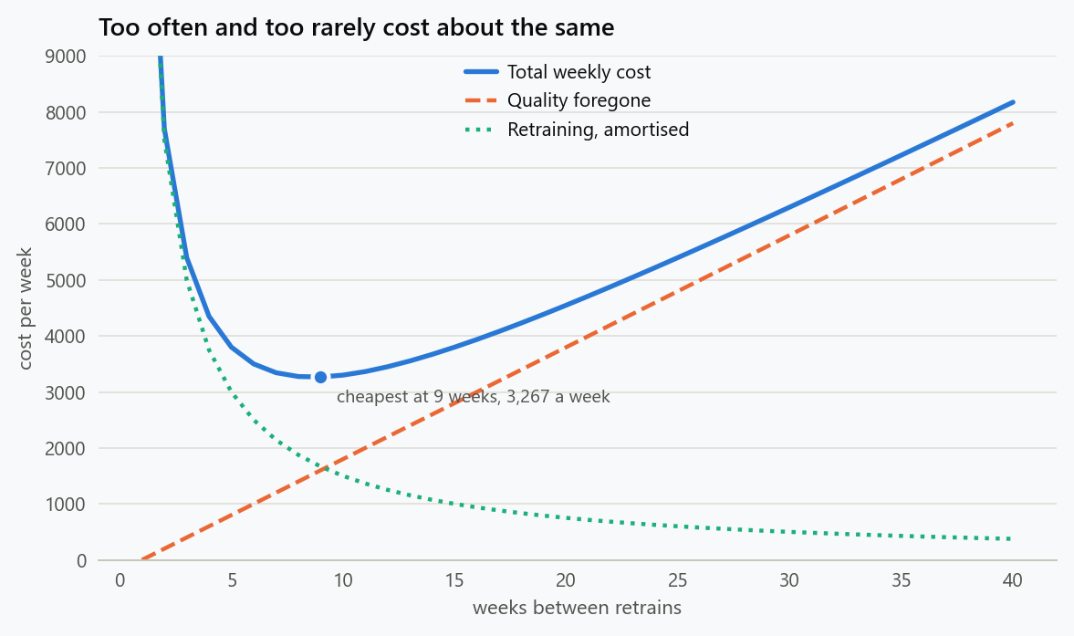
The cheapest schedule retrains every nine weeks at 3,267 a week. Fortnightly retraining costs 7,700 and annual retraining 10,488, both more than double the optimum, and weekly retraining costs 15,000 because nothing has decayed yet. The curve is flat near its minimum and steep away from it, which is the useful shape: anything between six and thirteen weeks is close to optimal here, and quarterly or weekly are both expensive.
Minimising the expression gives a rule worth remembering:
with $C$ the cost of a retraining, $\delta$ the quality lost per week of age and $V$ the value of a unit of quality. The numerical optimum of nine weeks matches the formula's 8.7.
1
2
3
4
5
for decay in (0.001, 0.004, 0.010):
    for cost in (5_000, 15_000, 50_000):
        b = min(range(1, 205), key=lambda p: schedule_cost(p, decay=decay, cost=cost))
        print(f"{decay:16.3f} {cost:14,.0f} {b:13d} "
              f"{schedule_cost(b, decay=decay, cost=cost):13,.0f}")
| Decay per week | Retraining cost | Best period | Weekly cost |
|---|---|---|---|
| 0.001 | 5,000 | 10 weeks | 950 |
| 0.001 | 15,000 | 17 weeks | 1,682 |
| 0.001 | 50,000 | 32 weeks | 3,112 |
| 0.004 | 5,000 | 5 weeks | 1,800 |
| 0.004 | 15,000 | 9 weeks | 3,267 |
| 0.004 | 50,000 | 16 weeks | 6,125 |
| 0.010 | 5,000 | 3 weeks | 2,667 |
| 0.010 | 15,000 | 5 weeks | 5,000 |
| 0.010 | 50,000 | 10 weeks | 9,500 |
Both inputs enter under a square root, which is why the answer is robust. Being wrong by a factor of four about the decay rate moves the interval by a factor of two, and the cost penalty for being within that range is small.
Triggering on Measured Quality
The alternative is to retrain when measured quality drops below a threshold. It sounds strictly better, since it responds to what is actually happening, and it inherits a problem: the measurement is noisy.
1
2
3
4
5
6
7
8
9
10
11
12
13
14
15
16
17
18
19
20
21
22
23
24
25
26
27
28
29
def run_trigger(threshold, noise, delay=0, decay=DECAY, weeks=WEEKS, rng=RNG):
    """Retrain when measured quality drops below `threshold`. Measurement is
    noisy and arrives `delay` weeks late."""
    age, total_cost, retrains, observed = 0, 0.0, 0, []
    for t in range(weeks):
        true_q = quality(age, decay)
        observed.append(true_q + rng.normal(0, noise))
        total_cost += VALUE * (1.0 - true_q)
        seen = observed[max(0, t - delay)]
        if seen < threshold:
            total_cost += COST
            retrains += 1
            age = 0
        else:
            age += 1
    return total_cost / weeks, retrains


for noise in (0.0, 0.005, 0.015):
    for threshold in (0.99, 0.98, 0.96):
        r = np.random.default_rng(5)
        costs, counts = [], []
        for _ in range(40):
            c, n = run_trigger(threshold, noise, rng=r)
            costs.append(c)
            counts.append(n)
        print(f"measurement noise {noise:5.3f}, trigger at {threshold:4.2f}: "
              f"weekly cost {np.mean(costs):9,.0f}, "
              f"{np.mean(counts) / (WEEKS / 52):4.1f} retrains a year")
| Measurement noise | Trigger at | Weekly cost | Retrains a year |
|---|---|---|---|
| 0.000 | 0.99 | 4,350 | 13.0 |
| 0.000 | 0.98 | 3,331 | 7.4 |
| 0.000 | 0.96 | 3,428 | 4.3 |
| 0.005 | 0.99 | 4,693 | 14.2 |
| 0.005 | 0.98 | 3,495 | 8.5 |
| 0.005 | 0.96 | 3,374 | 4.6 |
| 0.015 | 0.99 | 6,068 | 19.3 |
| 0.015 | 0.98 | 4,366 | 12.3 |
| 0.015 | 0.96 | 3,386 | 6.0 |
With a perfect signal, a trigger at 0.98 costs 3,331 a week, marginally better than the best schedule. Add realistic noise and it degrades, because a noisy measurement crosses the threshold early. At the tightest threshold, noise of 0.015 pushes the policy from 13 retrains a year to 19 and the cost from 4,350 to 6,068. The threshold that survives noise is the loose one, which is close to being a schedule in disguise.
Late Labels
The second problem is that quality is measured from labels, and labels arrive after the event. A four-week delay means the trigger fires on the state of the model a month ago.
1
2
3
4
5
6
7
8
9
for noise in (0.005, 0.015):
    for threshold in (0.99, 0.98):
        r = np.random.default_rng(7)
        costs = [run_trigger(threshold, noise, delay=4, rng=r)[0] for _ in range(40)]
        r2 = np.random.default_rng(7)
        costs0 = [run_trigger(threshold, noise, delay=0, rng=r2)[0] for _ in range(40)]
        print(f"noise {noise:5.3f}, trigger at {threshold:4.2f}: "
              f"no delay {np.mean(costs0):9,.0f}, four weeks late {np.mean(costs):9,.0f}, "
              f"{np.mean(costs) / np.mean(costs0) - 1:+6.1%}")
| Noise | Trigger at | No delay | Four weeks late | Change |
|---|---|---|---|---|
| 0.005 | 0.99 | 4,719 | 6,803 | +44.2% |
| 0.005 | 0.98 | 3,497 | 6,187 | +76.9% |
| 0.015 | 0.99 | 6,078 | 6,655 | +9.5% |
| 0.015 | 0.98 | 4,391 | 5,429 | +23.6% |
A month of label delay adds between a tenth and three quarters to the cost of the policy. The tighter the threshold, the worse the delay hurts, because the policy is trying to react quickly to something it can only see late. Any team whose labels take weeks to arrive should assume a trigger behaves like a schedule with a random period, and budget accordingly.
When a Trigger Is Actually Worth It
Comparing the best schedule against the best trigger under steady decay gives a result worth stating plainly.
1
2
3
4
5
6
7
8
9
10
11
12
for decay in (0.002, 0.004, 0.008):
    b = min(range(1, 205), key=lambda p: schedule_cost(p, decay=decay))
    sched = schedule_cost(b, decay=decay)
    r = np.random.default_rng(11)
    best_trigger = None
    for threshold in np.arange(0.90, 0.999, 0.005):
        costs = [run_trigger(threshold, 0.005, decay=decay, rng=r)[0] for _ in range(20)]
        if best_trigger is None or np.mean(costs) < best_trigger[1]:
            best_trigger = (threshold, np.mean(costs))
    print(f"decay {decay:5.3f}: best schedule every {b:3d} weeks at {sched:9,.0f}, "
          f"best trigger at {best_trigger[0]:4.2f} costing {best_trigger[1]:9,.0f}, "
          f"{best_trigger[1] / sched - 1:+6.1%}")
| Decay per week | Best schedule | Best trigger | Difference |
|---|---|---|---|
| 0.002 | every 12 weeks, 2,350 | at 0.98, 2,361 | +0.5% |
| 0.004 | every 9 weeks, 3,267 | at 0.97, 3,275 | +0.3% |
| 0.008 | every 6 weeks, 4,500 | at 0.97, 4,514 | +0.3% |
When decay is steady, a well-chosen schedule and a well-tuned trigger cost the same to within half a percent, and the schedule is simpler, cheaper to operate and easier to plan around. That is the opposite of how the choice is usually argued.
The case for a trigger is not steady decay. It is the possibility of an abrupt drop that a schedule cannot anticipate.
1
2
3
4
5
6
7
8
9
10
11
12
13
14
15
16
17
18
19
20
21
22
23
24
25
26
27
28
def run_mixed(policy, threshold=0.98, period=9, noise=0.005, shock=0.05,
              shock_rate=1 / 40, weeks=WEEKS, rng=RNG):
    """Steady decay plus occasional abrupt drops that a schedule cannot anticipate."""
    age, deficit, total, retrains = 0, 0.0, 0.0, 0
    for t in range(weeks):
        if rng.random() < shock_rate:
            deficit += shock
        true_q = quality(age) - deficit
        total += VALUE * (1.0 - true_q)
        fire = (age + 1 >= period) if policy == "schedule" else \
               (true_q + rng.normal(0, noise) < threshold)
        if fire:
            total += COST
            retrains += 1
            age, deficit = 0, 0.0
        else:
            age += 1
    return total / weeks, retrains


for shock_rate in (0, 1 / 80, 1 / 40, 1 / 20):
    r = np.random.default_rng(13)
    sched = [run_mixed("schedule", shock_rate=shock_rate, rng=r)[0] for _ in range(40)]
    r = np.random.default_rng(13)
    trig = [run_mixed("trigger", shock_rate=shock_rate, rng=r)[0] for _ in range(40)]
    label = "never" if shock_rate == 0 else f"every {1 / shock_rate:.0f} weeks on average"
    print(f"shocks {label:28s}: schedule {np.mean(sched):9,.0f}, "
          f"trigger {np.mean(trig):9,.0f}, {np.mean(trig) / np.mean(sched) - 1:+6.1%}")
| Abrupt drops arrive | Schedule | Trigger | Difference |
|---|---|---|---|
| Never | 3,239 | 3,502 | +8.1% |
| Every 80 weeks | 3,567 | 3,619 | +1.5% |
| Every 40 weeks | 3,847 | 3,757 | −2.4% |
| Every 20 weeks | 4,474 | 4,027 | −10.0% |
The crossover sits around one shock every forty weeks. Below that the schedule wins because it never retrains for a measurement artefact. Above it the trigger wins because the schedule spends weeks running a model that broke on a Tuesday.
That gives a rule for choosing between them: count the abrupt breaks in the last two years. If the answer is none, a schedule is the cheaper and simpler policy. If the answer is several, a trigger pays for itself, and the priority becomes making the quality signal fast and quiet rather than tuning the threshold.
Estimating the Two Inputs
Both quantities that set the schedule are measurable from history. The decay rate comes from evaluating a fixed model against successive weeks of held-out data and fitting a slope to the result; the exercise takes an afternoon and is worth repeating yearly. The retraining cost is compute plus the human time of review and deployment, and teams usually underestimate the second, which pushes the optimal interval longer than instinct suggests.
The value of a unit of quality is the one that requires a conversation rather than a query. It is also the one the answer is least sensitive to, because it sits under a square root alongside the decay rate.
What to Do
- Measure the decay rate before choosing a cadence: evaluate one frozen model against successive weeks and fit the slope.
- Use the square-root rule as the starting point, and remember the cost curve is flat near its minimum, so any interval within a factor of about one and a half is fine.
- Count the real retraining cost, including review and deployment time. Underestimating it makes you retrain too often.
- Prefer a schedule when decay is steady. Under these assumptions the best trigger saves nothing and costs more to operate.
- Use a trigger when abrupt breaks are common, roughly more than one a year, and then invest in a fast, low-noise quality signal rather than in threshold tuning.
- Add the label delay to any trigger's expected reaction time, and treat a delayed trigger as a schedule with an unpredictable period.
The figure generator in the blog-reproducibility repository reproduces this article's figure; run it with --dry-run to print the numbers behind the figure without writing an image.
References
- Gama, J., Žliobaitė, I., Bifet, A., Pechenizkiy, M., & Bouchachia, A. (2014). A survey on concept drift adaptation. ACM Computing Surveys, 46(4), 1-37.
- Bifet, A., & Gavaldà, R. (2007). Learning from time-changing data with adaptive windowing. Proceedings of the 2007 SIAM International Conference on Data Mining, 443-448.
- Sculley, D., Holt, G., Golovin, D., Davydov, E., Phillips, T., Ebner, D., Chaudhary, V., Young, M., Crespo, J.-F., & Dennison, D. (2015). Hidden technical debt in machine learning systems. Advances in Neural Information Processing Systems, 28, 2503-2511.
- Barlow, R. E., & Proschan, F. (1965). Mathematical Theory of Reliability. Wiley.
- Harrison, P. J., & Davies, O. L. (1964). The use of cumulative sum (cusum) techniques for the control of routine forecasts of product demand. Operations Research, 12(2), 325-333.
- Klinkenberg, R., & Joachims, T. (2000). Detecting concept drift with support vector machines. Proceedings of the Seventeenth International Conference on Machine Learning, 487-494.
Embed interactive plots, widgets, and demos using <figure>, <iframe>, or <div class="interactive-embed"> containers. Ensure each embed includes descriptive captions for accessibility.
How to cite
Use the quick export buttons to save citations for reference managers or copy the formatted text directly.
Diogo Ribeiro (2026). How Often to Retrain: A Square-Root Rule and Its Limits. Faculty of Media Arts and Design, Technical University of Porto. https://diogoribeiro7.github.io/machine-learning/how_often_to_retrain_a_model/.