Topics
The Monday report says sign-ups are down six percent week over week. A channel owner is asked to explain it. By Thursday the number is up four percent and nobody mentions it again.
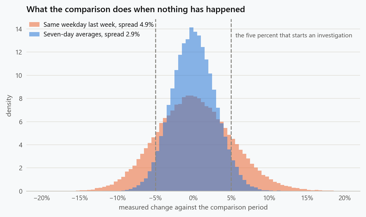
Both movements are noise, and the size of that noise is measurable in advance. On a metric with ordinary weekday seasonality and ordinary day-to-day persistence, comparing a day against the same weekday last week has a spread of about five percent when nothing whatsoever has changed.
What the Comparison Does on a Quiet Metric
The simulation builds a daily metric with a weekday pattern, autocorrelated noise and no real change at all, then applies three comparisons that appear in every operational report.
1
2
3
4
5
6
7
8
9
10
11
12
13
14
15
16
17
18
19
20
21
22
23
24
25
26
27
28
29
30
31
32
33
34
35
36
37
38
39
40
41
42
43
44
45
46
47
48
49
50
51
import numpy as np

RNG = np.random.default_rng(83)
DAYS = 560
LEVEL = 1000.0
WEEKDAY = np.array([1.05, 1.08, 1.06, 1.04, 1.10, 0.82, 0.85])   # Mon to Sun
RHO, SD = 0.55, 0.035                                            # day-to-day noise


def series(days=DAYS, step_at=None, step=0.0, rng=RNG):
    """A daily metric with weekday seasonality, autocorrelated noise and an
    optional permanent step change."""
    eps = rng.normal(0, SD * np.sqrt(1 - RHO ** 2), days)
    z = np.zeros(days)
    for i in range(1, days):
        z[i] = RHO * z[i - 1] + eps[i]
    level = np.full(days, LEVEL)
    if step_at is not None:
        level[step_at:] *= (1 + step)
    return level * WEEKDAY[np.arange(days) % 7] * (1 + z)


def wow_day(y, t):
    """Today against the same weekday last week."""
    return y[t] / y[t - 7] - 1


def wow_mean(y, t, w=7):
    """The last seven days against the seven before them."""
    return y[t - w + 1:t + 1].mean() / y[t - 2 * w + 1:t - w + 1].mean() - 1


def yoy_day(y, t):
    """Today against the nearest same weekday a year earlier."""
    return y[t] / y[t - 364] - 1


r = np.random.default_rng(3)
d1, d7, dyy = [], [], []
for _ in range(400):
    y = series(rng=r)
    for t in range(400, DAYS):
        d1.append(wow_day(y, t))
        d7.append(wow_mean(y, t))
        dyy.append(yoy_day(y, t))
for name, v in (("same weekday last week", d1), ("seven-day averages", d7),
                ("same weekday last year", dyy)):
    v = np.array(v)
    print(f"{name:24s} spread {v.std():6.2%}, "
          f"exceeds 5% in {np.mean(np.abs(v) > 0.05):5.1%} of days, "
          f"exceeds 10% in {np.mean(np.abs(v) > 0.10):5.1%}")
| Comparison | Spread | Exceeds 5% | Exceeds 10% |
|---|---|---|---|
| Same weekday last week | 4.93% | 30.8% of days | 4.3% |
| Seven-day averages | 2.86% | 8.0% | 0.1% |
| Same weekday last year | 4.93% | 30.8% | 4.2% |
A five percent movement week over week happens on three days in ten with nothing behind it. A ten percent movement happens about once a month. The year-over-year comparison behaves identically, because it removes the same weekday pattern and replaces one noisy day with another noisy day.
1
2
3
4
5
6
for name, v in (("same weekday last week", d1), ("seven-day averages", d7),
                ("same weekday last year", dyy)):
    v = np.array(v)
    print(f"{name:24s} a 5% false alarm rate needs a threshold of "
          f"{np.quantile(np.abs(v), 0.95):5.2%}, a 1% rate needs "
          f"{np.quantile(np.abs(v), 0.99):5.2%}")
| Comparison | Threshold for a 5% false alarm rate | For a 1% rate |
|---|---|---|
| Same weekday last week | 9.63% | 12.86% |
| Seven-day averages | 5.58% | 7.36% |
| Same weekday last year | 9.65% | 12.84% |
Those are the numbers a reporting convention should carry. If the rule is "investigate anything over five percent", the honest version of that rule on a single-day comparison is "investigate anything over ten percent", and the honest version on weekly averages is "over five and a half".
The Same Rules, Made Comparable
Comparing detection speed only means something once every rule has the same appetite for false alarms. Here each is tuned so that a quiet four-week window trips it one time in ten.
1
2
3
4
5
6
7
8
9
10
11
12
13
14
15
16
17
18
19
20
21
22
23
24
25
26
27
28
29
30
31
32
33
34
35
36
37
38
39
40
41
42
43
44
45
46
STEP_AT = 450
WINDOW = 28


def rules(y, thresholds):
    """Each rule as a function of the day index, at its own threshold."""
    pattern = np.array([y[:STEP_AT - 20][np.arange(STEP_AT - 20) % 7 == k].mean()
                        for k in range(7)])
    adj = y / pattern[np.arange(len(y)) % 7]
    base = adj[200:STEP_AT - 20]
    return {
        "same weekday": lambda t: abs(wow_day(y, t)) > thresholds["same weekday"],
        "seven-day means": lambda t: abs(wow_mean(y, t)) > thresholds["seven-day means"],
        "seasonal residual": lambda t: (abs(adj[t] - base.mean())
                                        > thresholds["seasonal residual"] * base.std()),
    }


def false_alarm_rate(thresholds, runs=200, seed=7):
    r = np.random.default_rng(seed)
    hits = {k: 0 for k in thresholds}
    for _ in range(runs):
        y = series(rng=r)
        fns = rules(y, thresholds)
        for k, fn in fns.items():
            hits[k] += any(fn(t) for t in range(STEP_AT, STEP_AT + WINDOW))
    return {k: v / runs for k, v in hits.items()}


# Tune each threshold until a quiet four-week window trips it one time in ten.
thresholds = {"same weekday": 0.10, "seven-day means": 0.06, "seasonal residual": 3.0}
for key, lo, hi in (("same weekday", 0.05, 0.40), ("seven-day means", 0.02, 0.30),
                    ("seasonal residual", 1.5, 6.0)):
    for _ in range(12):
        mid = (lo + hi) / 2
        trial = dict(thresholds, **{key: mid})
        if false_alarm_rate(trial, runs=120)[key] > 0.10:
            lo = mid
        else:
            hi = mid
    thresholds[key] = (lo + hi) / 2
rates = false_alarm_rate(thresholds, runs=300)
for k, v in thresholds.items():
    unit = "standard deviations" if k == "seasonal residual" else "percent"
    shown = f"{v:.2f} {unit}" if k == "seasonal residual" else f"{v:.2%}"
    print(f"{k:18s} threshold {shown:24s} false alarms {rates[k]:5.1%} per quiet month")
| Rule | Threshold for one false alarm per ten quiet months | Measured false alarm rate |
|---|---|---|
| Same weekday last week | 14.22% | 11.3% |
| Seven-day averages | 7.91% | 9.0% |
| Seasonal residual | 3.14 standard deviations | 7.7% |
A week-over-week rule that fires as rarely as a three-sigma control chart has to ignore anything under fourteen percent. That is the practical cost of comparing two single noisy days: the rule becomes either constantly wrong or nearly deaf.
1
2
3
4
5
6
7
8
9
10
11
12
13
14
15
16
17
for step in (0.02, 0.03, 0.05, 0.10):
    r = np.random.default_rng(5)
    found = {k: [] for k in thresholds}
    for _ in range(300):
        y = series(step_at=STEP_AT, step=step, rng=r)
        fns = rules(y, thresholds)
        for k, fn in fns.items():
            hit = next((t - STEP_AT for t in range(STEP_AT, DAYS) if fn(t)), None)
            found[k].append(hit if hit is not None else DAYS - STEP_AT)
    parts = []
    for k, v in found.items():
        v = np.array(v)
        seen = v < 28
        median = np.median(v[seen]) if seen.any() else float("nan")
        parts.append(f"{k} {seen.mean():5.1%} within four weeks"
                     + (f", median {median:4.1f} days" if seen.any() else ""))
    print(f"step of {step:4.0%}: " + "; ".join(parts))
| Real step | Same weekday catches it | Seven-day means | Seasonal residual |
|---|---|---|---|
| 2% | 16.3% within four weeks | 12.0% | 16.7% |
| 3% | 22.0% | 15.7% | 34.7% |
| 5% | 32.3% | 33.0% | 72.3% |
| 10% | 72.0% | 82.0% | 100.0% |
At a matched false alarm rate the seasonal residual catches a five percent step 72 percent of the time within four weeks, against about a third for either period comparison. The gap widens at three percent and closes only at ten, where everything works.
The reason is not sophistication. The residual compares today against a model of what today should look like, built from hundreds of days, while a week-over-week comparison compares today against exactly one day, chosen for sharing a weekday and nothing else.
Seven Days Is Not Seven Times Better
A natural response is to average the week, which helps, but less than the arithmetic of independent observations promises.
1
2
3
4
5
6
7
8
9
10
r = np.random.default_rng(11)
singles, means = [], []
for _ in range(2000):
    y = series(days=120, rng=r)
    singles.append(wow_day(y, 100))
    means.append(wow_mean(y, 100))
print(f"single day comparison spread {np.std(singles):.3%}")
print(f"seven-day average comparison spread {np.std(means):.3%}")
print(f"ratio {np.std(singles) / np.std(means):.2f}, against {np.sqrt(7):.2f} "
      f"if the days were independent")
| Quantity | Value |
|---|---|
| Spread of a single-day comparison | 4.925% |
| Spread of a seven-day average comparison | 2.821% |
| Ratio | 1.75 |
| Ratio if days were independent | 2.65 |
Averaging seven correlated days buys a factor of 1.75 rather than 2.65. Days near each other share conditions, so the seventh day adds much less information than the first, and the same persistence means the two windows being compared are themselves correlated. Any calculation that treats daily observations as independent will overstate the precision of a weekly figure by about half.
What to Report Instead
None of this argues against showing week-over-week numbers. It argues against showing them alone, with a fixed percentage threshold attached.
Three changes cover most of the gap. Put an interval on the comparison, computed from the metric's own history rather than from a formula that assumes independence. Compare against a seasonal expectation, which needs nothing more than an average by weekday and a level estimate. And reserve investigation for movements that the metric's own noise does not readily produce, which the first table gives directly: for this metric, about ten percent on a single day and five and a half on a weekly average.
What to Do
- Measure the spread of your own comparison on a quiet period before setting any threshold. One query over the last year gives it.
- Publish that spread next to the comparison, so a reader can tell an unusual movement from an ordinary one.
- Prefer a seasonal residual to a period comparison for anything that triggers work. At the same false alarm rate it catches a five percent step twice as often.
- Treat year-over-year on a single day as no more reliable than week-over-week. It removes the same seasonality and adds a year of drift.
- Do not assume a weekly average is the square root of seven times more precise. With day-to-day persistence the real factor here is 1.75.
- Escalate on persistence rather than on a single reading. A step that is real will still be there next week, and a metric that moves once will usually move back.
The figure generator in the blog-reproducibility repository reproduces this article's figure; run it with --dry-run to print the numbers behind the figure without writing an image.
References
- Box, G. E. P., Jenkins, G. M., Reinsel, G. C., & Ljung, G. M. (2015). Time Series Analysis: Forecasting and Control (5th ed.). Wiley.
- Cleveland, R. B., Cleveland, W. S., McRae, J. E., & Terpenning, I. (1990). STL: a seasonal-trend decomposition procedure based on loess. Journal of Official Statistics, 6(1), 3-73.
- Montgomery, D. C. (2019). Introduction to Statistical Quality Control (8th ed.). Wiley.
- Alwan, L. C., & Roberts, H. V. (1988). Time-series modeling for statistical process control. Journal of Business and Economic Statistics, 6(1), 87-95.
- Hyndman, R. J., & Athanasopoulos, G. (2021). Forecasting: Principles and Practice (3rd ed.). OTexts.
- Bartlett, M. S. (1946). On the theoretical specification and sampling properties of autocorrelated time-series. Supplement to the Journal of the Royal Statistical Society, 8(1), 27-41.
Embed interactive plots, widgets, and demos using <figure>, <iframe>, or <div class="interactive-embed"> containers. Ensure each embed includes descriptive captions for accessibility.
How to cite
Use the quick export buttons to save citations for reference managers or copy the formatted text directly.
Diogo Ribeiro (2026). Week Over Week: A Comparison That Moves Five Percent on Its Own. Faculty of Media Arts and Design, Technical University of Porto. https://diogoribeiro7.github.io/statistics/week_over_week_comparisons/.


