Topics
A 95% confidence interval that runs from $-71.7$ to $2.53$, for the mean of a Gaussian with unit variance, looks like a bug. If I saw it come out of my own code I would check the root finder, the tail probabilities and the sign conventions before believing it. Yet it is the exact answer to a well-posed question, and the procedure that produced it covers the true mean 95% of the time, as it promises.
The question is what a selected observation says about its mean once we admit that it was reported because it was large. Conditioning on the selection is what makes the interval honest, and it is also what can make it enormous. This article works one example all the way through: the exact interval, a closed form for how fast it widens, the reason its expected width is infinite, how badly the ordinary interval does in the same setting, and two ways of paying less.
One Observation and a Reporting Rule
Let $X \sim N(\mu, 1)$, and suppose we report $X$ only when $X > 2$. This is the smallest possible model of a screening step. We look at many candidates, keep the ones that clear a bar, and then want an interval for what we kept. Suppose the observation is $x = 2.05$.
Ignoring the rule, the ordinary interval is $2.05 \pm 1.96$, or $[0.09, 4.01]$. It excludes zero, it is as narrow as any interval for this problem can be, and it is wrong in a specific way: it describes the behaviour of $X$ over all repetitions of the experiment, while we only ever see the repetitions in which $X$ exceeded 2. Over those, the relevant distribution is the normal truncated to $(2, \infty)$. Writing $\bar\Phi = 1 - \Phi$ for the Gaussian survival function, its distribution function $F_\mu(x) = P_\mu(X \le x \mid X > 2)$ is, for $x > 2$,
Under the true mean, $F_\mu(X)$ is uniform on $(0, 1)$ given selection, and $F_\mu(x)$ falls as $\mu$ rises, because a larger mean makes any fixed $x$ sit lower in its conditional distribution. Those two facts are all an exact interval needs. The equal-tailed 95% limits are the means at which the observed value sits at the two extreme quantiles,
For $x = 2.05$ they are $\mu_L = -71.74$ and $\mu_U = 2.53$. The table repeats the calculation for observations further above the bar.
| Observed $x$ | Above 2 | Ordinary | Exact selective | Width |
|---|---|---|---|---|
| 2.01 | 0.01 | [0.05, 3.97] | [-366.88, -0.17] | 366.7 |
| 2.05 | 0.05 | [0.09, 4.01] | [-71.74, 2.53] | 74.3 |
| 2.20 | 0.20 | [0.24, 4.16] | [-16.29, 3.66] | 19.9 |
| 2.50 | 0.50 | [0.54, 4.46] | [-4.99, 4.31] | 9.3 |
| 3.00 | 1.00 | [1.04, 4.96] | [-0.93, 4.93] | 5.9 |
| 3.50 | 1.50 | [1.54, 5.46] | [0.66, 5.46] | 4.8 |
| 5.00 | 3.00 | [3.04, 6.96] | [2.96, 6.96] | 4.0 |
Two things stand out. The upper limits of the two intervals agree from about $x = 3$ onwards, and by $x = 5$ the intervals are nearly identical: far from the threshold, selection hardly matters, because the observation would have been reported under any plausible mean. All the damage is in the lower limit, and it is governed by the distance above the threshold, not by the size of the observation. At $x = 2.01$ the interval does not even contain the observation.
Why the Lower Limit Runs Away
A very negative mean makes the event $X > 2$ absurdly unlikely. At $\mu = -71.74$ its probability is about $10^{-1183}$. But the interval is built from the distribution given that event, and given that event a very negative mean makes a sharp prediction: the observation will be found just above 2. The reason is the shape of the Gaussian tail. For large $t$, the ratio $\bar\Phi(t + d) / \bar\Phi(t)$ behaves like $e^{-td}$, so with $t = 2 - \mu$ and $d = x - 2$ the excess over the threshold is approximately exponential with rate $2 - \mu$:
At $\mu = -20$ that is an exponential with mean $0.045$, and $x = 2.05$ sits at its 67th percentile: unremarkable. At $\mu = 1$ the same observation sits at the 7th percentile, which is also unremarkable. The left panel of the figure shows the three conditional densities. A value of 2.05 is compatible with all of them, so it cannot tell them apart, and that is precisely what the interval reports.
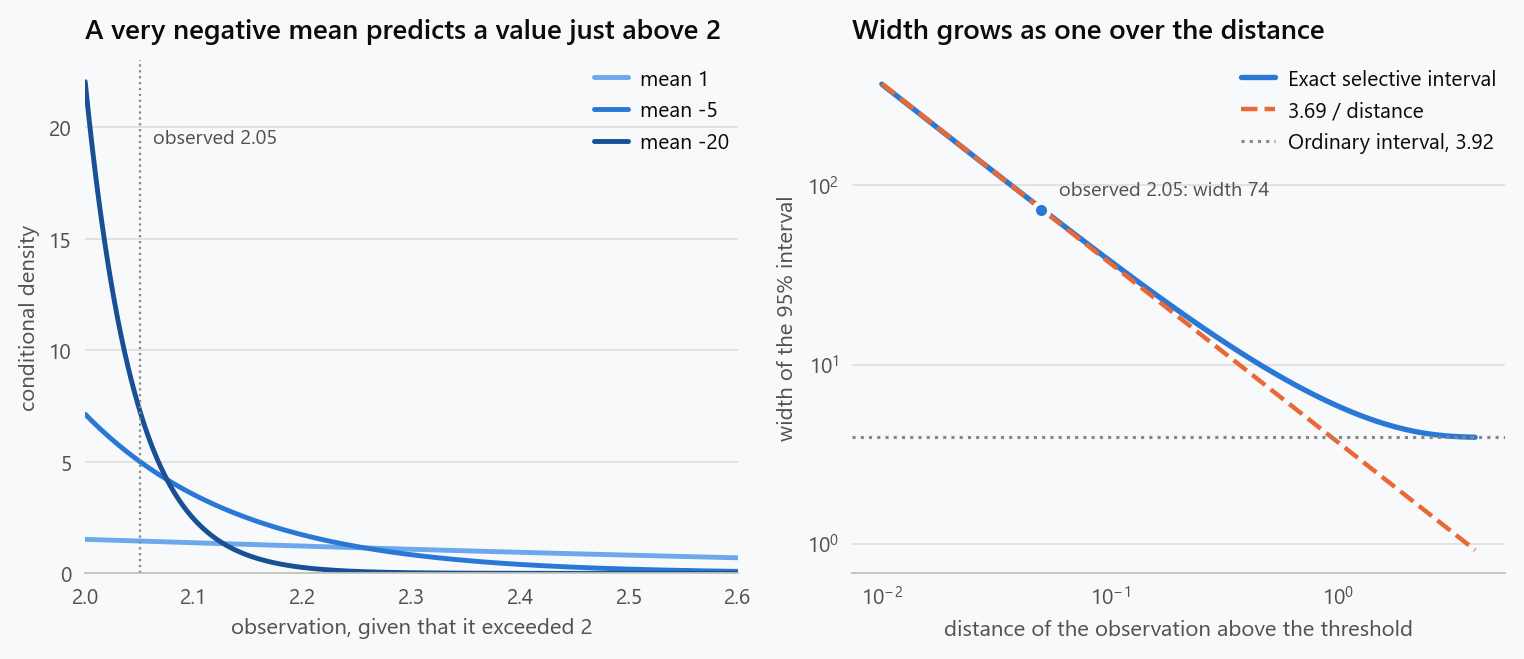
Setting the approximation equal to $1 - \alpha/2$ and solving for the mean gives the lower limit in closed form, for a threshold $c$ and an observation at distance $d = x - c$ above it,
where $\ln(2/\alpha) = 3.69$ at the 95% level. For $x = 2.05$ this gives $-71.78$ against the exact $-71.74$; for $x = 2.01$, $-366.89$ against $-366.88$; for $x = 2.2$, $-16.44$ against $-16.29$. It degrades as the distance grows, as it should, since the exponential tail is a statement about means far below the threshold. The right panel of the figure shows the exact width staying within 10% of $3.69/d$ from $d = 0.01$ to about $d = 0.2$, widths from 367 down to 20, before bending towards the ordinary width of $3.92$.
This is the whole phenomenon in one line. The information that would have ruled out $\mu = -72$ is the improbability of crossing the threshold at all, and conditioning on the crossing removes exactly that information from the calculation. What remains is where the observation landed inside the selection region, and a landing $0.05$ above the edge is what almost every mean below the edge predicts.
The Expected Width Is Infinite
The width is roughly $3.69/d$ when the distance $d$ is small. How often is it small? Given selection, the density of $X$ at the threshold is the Gaussian hazard $h(2 - \mu) = \phi(2 - \mu) / \bar\Phi(2 - \mu)$, which is strictly positive for every mean. So $d$ has a density that does not vanish at zero, and for large $w$ the width has a tail that decays only as the reciprocal of its argument:
A tail of order $1/w$ has no mean. The expected width of the exact interval is infinite, for every value of $\mu$, even though every individual interval is finite. Kivaranovic and Leeb (2021) prove this in general for intervals built by conditioning on polyhedral selection events. Their Proposition 1 states that whenever the truncation region is bounded from above or from below the expected length is infinite, for the reason just given. They also show that the upper quantiles of the length grow like $1/(1 - \kappa)$ as the level $\kappa$ approaches 1, which is the same $1/w$ tail read the other way round. For the lasso they find the condition met in most of the problems they simulate, the exceptions being models that contain almost all or almost none of the regressors.
Under $\mu = 0$ the hazard at the threshold is $2.37$, so the approximation reads $8.75/w$. The exact limit is slightly smaller, $8.69/w$, because the upper end of the interval recedes as well, by $\ln(1/0.975)/d$, so that near the threshold the width is $\ln(39)/d = 3.66/d$ rather than $3.69/d$. The exact quantiles of the width, given selection, bear it out. The second column is the probability of selection and the last the share of intervals wider than 20.
| Mean | Selected | Median | 90th | 99th | Over 20 |
|---|---|---|---|---|---|
| 0 | 0.023 | 14.96 | 84.1 | 865.9 | 38.8% |
| 1 | 0.159 | 10.85 | 55.1 | 557.1 | 27.4% |
| 2 | 0.500 | 7.51 | 30.6 | 292.7 | 15.8% |
| 3 | 0.841 | 5.32 | 13.9 | 108.0 | 6.3% |
| 4 | 0.977 | 4.31 | 6.6 | 25.1 | 1.3% |
These are not simulation artefacts. Because the width is a decreasing function of the observation, its quantiles follow exactly from the quantiles of the truncated normal, and a simulation of 20,000 selected draws per row reproduces them while confirming coverage between 94.6% and 95.3%. The sample mean of the simulated widths, by contrast, never settles: it was 88 at $\mu = 0$ in one run, driven by a single interval more than 100,000 wide.
I first met this in a stress test of a selective-inference implementation, not in a toy model. On null data with 40 observations, 1,000 draws gave a median width of 4.7, a 90th percentile of 23.8 and a maximum of 5,817.9, with about one interval in eight wider than 20 standard deviations. The root finding was stable, the selection event was right and the calibration was correct. The widest intervals belonged, without exception, to the most marginal selections.
What the Ordinary Interval Gets Wrong
It is tempting to look at $[-71.7, 2.53]$, call the exact method too conservative, and report $[0.09, 4.01]$ instead. The ordinary interval covers $\mu$ when $\lvert X - \mu \rvert \le 1.96$, and given selection the probability of that is easy to write down. The table gives the coverage of $X \pm 1.96$ among reported observations.
| Mean | Coverage, given $X > 2$ |
|---|---|
| 0 or below | 0% |
| 0.5 | 62.6% |
| 1 | 84.2% |
| 1.5 | 91.9% |
| 2 | 95.0% |
| 3 | 97.0% |
For any mean below $0.04$ the coverage is not low, it is zero. The interval contains $\mu$ only when $X < \mu + 1.96$, and a reported $X$ is always above 2, so when $\mu + 1.96 < 2$ the two conditions cannot both hold. Every interval reported under the null excludes the truth, and every one of them excludes zero. This is the winner's curse in its purest form (Zhong and Prentice, 2008). The same fluctuation is used twice: once to get the observation selected, and again as if it were fresh evidence about the mean.
The over-coverage at $\mu = 3$ is the other side of the same coin and is harmless. The point of the table is that the ordinary interval's 95% is a statement about all repetitions, and nobody reads the ones that were not reported.
Search Creates the Same Geometry
Nothing above depends on the threshold being fixed in advance. Lee, Sun, Sun and Taylor (2016) showed that for the lasso, and for many other procedures, the event "this model was selected, with these signs" is a set of linear inequalities ${Ay \le b}$ in the response. Conditional on that event, and on the part of the data orthogonal to the contrast of interest, a linear contrast $\eta^\top y$ is a Gaussian truncated to an interval $[\mathcal{V}^-, \mathcal{V}^+]$ whose ends are computed from $A$, $b$ and the data. Inference then inverts the same pivot as in equation $\eqref{eq:cdf}$, with a data-dependent truncation region in place of $(2, \infty)$.
The distance $d$ becomes the gap between the observed contrast and the nearer end of its truncation interval. When the search picks the largest of $m$ statistics, that gap is essentially the margin by which the winner beat the runner-up. When a changepoint algorithm picks a break location, it is the margin by which that location beat its neighbours (Hyun, Lin, G'Sell and Tibshirani, 2021). A winner that barely won is the multidimensional version of observing 2.05 after requiring more than 2, and equation $\eqref{eq:limit}$ says what to expect: a limit that recedes as the reciprocal of the margin.
This is why a narrow interval after a weak search result should make a reader more suspicious, not less. If a break is chosen as the most extreme of several hundred candidate locations, and the reported interval is as tight as if the location had been fixed beforehand, the likeliest explanation is that the search was ignored.
Paying Less: Randomisation and Splitting
The exact interval is wide because conditioning on ${X > 2}$ throws away all the information carried by the selection event, and for a marginal selection that was nearly all the information there was. Fithian, Sun and Taylor (2014) call what remains the leftover information, and they observe that how much remains is a design choice. Two designs leave more.
The first is data splitting: select with one independent half of the data and infer with the other. If $X$ is the mean of the whole sample, each half has variance 2, the selection event says nothing about the inference half, and the interval is an ordinary one of width $2 \times 1.96 \times \sqrt{2} = 5.54$, whatever happened at the selection stage. The second is randomised selection (Tian and Taylor, 2018): select on a noisy copy, $X + \omega > 2$ with $\omega \sim N(0, \gamma^2)$ drawn by the analyst, and infer from $X$ given that event. The conditional density of $X$ is then proportional to
a smooth reweighting in place of a hard cut. No value of $x$ sits on an edge, so no limit runs away. With $\gamma = 1$, which spends the same information on selection as an even split, the interval at $x = 2.05$ is $[-1.31, 3.60]$: width $4.92$ where the hard threshold gave $74.3$.
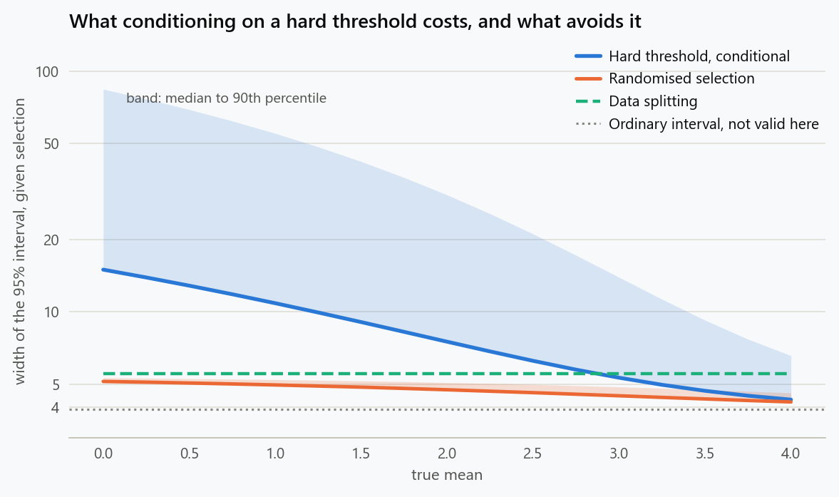
The figure shows the median width of each procedure, given selection, with a band up to its 90th percentile. The table gives the same numbers, together with the share of experiments that each selection rule reports.
| Mean | Selected: hard / rand. | Hard: median, 90th | Randomised: median, 90th | Split |
|---|---|---|---|---|
| 0 | 2.3% / 7.9% | 14.96, 84.1 | 5.13, 5.31 | 5.54 |
| 1 | 15.9% / 24.0% | 10.85, 55.1 | 4.96, 5.22 | 5.54 |
| 2 | 50.0% / 50.0% | 7.51, 30.6 | 4.74, 5.08 | 5.54 |
| 3 | 84.1% / 76.0% | 5.32, 13.9 | 4.47, 4.87 | 5.54 |
| 4 | 97.7% / 92.1% | 4.31, 6.6 | 4.22, 4.60 | 5.54 |
All three procedures cover 95% given selection; in the simulation behind the randomised column their coverage ranged from 94.4% to 95.5% across the fifteen cells. The randomised interval was never wider than $5.51$ for observations from $-4$ to $10$, and for observations further down its width creeps up towards the splitting width of $5.54$ without reaching it, which is an instance of a general result: Kivaranovic and Leeb (2020) show that randomised selection and data carving give intervals of bounded length that are never longer than the corresponding split.
None of this is free, and the second column shows where the bill goes. Randomising the selection changes what gets selected: under the null it reports more than three times as many false leads, and at $\mu = 4$ it misses 8% of real effects where the hard threshold misses 2%. Splitting pays the same price in a different coin. The choice is between a sharp selection with occasionally useless intervals and a blunter selection with uniformly usable ones, and which is better depends on whether the selection or the interval is the product. Rasines and Young (2023) compare the splitting strategies directly. A third route avoids conditioning altogether: simultaneous inference over every model the search could have chosen (Berk et al., 2013) is valid whatever the selection rule, at the price of intervals that are wider for every result, the clear winners included.
What Software Should Do With This
An implementation has to keep two things apart that look alike in the output. A numerical failure is a root finder that cannot bracket a solution, a probability that comes back as NaN, an interval that changes under a harmless rescaling, or two equivalent formulations that disagree. A statistically uninformative result is a correct interval of $[-3000, 3000]$. The first needs a fix; the second needs to be reported as it is, with its cause.
The numerical side is mostly one decision. The textbook form of the pivot, $(\Phi(x - \mu) - \Phi(2 - \mu)) / (1 - \Phi(2 - \mu))$, is unusable where the limits actually live: at $\mu = -71.74$ both distribution functions round to 1 and the expression evaluates to 0.0 / 0.0. The ratio of survival functions in equation $\eqref{eq:cdf}$, computed from their logarithms, is exact there. The bracket for the root also has to be allowed to grow, since a fixed search range silently turns a limit of $-366$ into a failure.
1
2
3
4
5
6
7
8
9
10
11
12
13
14
15
16
17
18
19
20
21
22
23
24
25
26
27
28
29
30
31
import numpy as np
from scipy.optimize import brentq
from scipy.stats import norm

THRESHOLD = 2.0


def conditional_cdf(mu, x, c=THRESHOLD):
    """P(X <= x | X > c) for X ~ N(mu, 1), from log survival functions."""
    return -np.expm1(norm.logsf(x - mu) - norm.logsf(c - mu))


def limit(target, x, c=THRESHOLD):
    """The mean at which the conditional cdf of x equals `target`."""
    f = lambda mu: conditional_cdf(mu, x, c) - target
    low, high = x - 1.0, x + 1.0
    while f(low) < 0:            # the cdf falls as the mean rises
        low -= 2 * (x - low)
    while f(high) > 0:
        high += 2 * (high - x)
    return brentq(f, low, high, xtol=1e-12)


def selective_interval(x, alpha=0.05):
    return limit(1 - alpha / 2, x), limit(alpha / 2, x)


for x in (2.05, 2.5, 3.0, 3.5):
    low, high = selective_interval(x)
    approx = THRESHOLD - np.log(40) / (x - THRESHOLD)
    print(f"x = {x:4.2f}   [{low:7.2f}, {high:5.2f}]   tail approximation {approx:7.2f}")
1
2
3
4
x = 2.05   [ -71.74,  2.53]   tail approximation  -71.78
x = 2.50   [  -4.99,  4.31]   tail approximation   -5.38
x = 3.00   [  -0.93,  4.93]   tail approximation   -1.69
x = 3.50   [   0.66,  5.46]   tail approximation   -0.46
The statistical side is about what is shown to the user. Report the margin of selection next to every interval: the distance above the threshold here, the gap to the runner-up in a search. It explains at a glance why two selected effects of the same size carry such different uncertainty, and with equation $\eqref{eq:limit}$ it predicts the width before it is computed. Do not clip an interval to make a plot readable without marking the clipped end and giving the true limit in a table, because a clipped interval is a different inferential statement. And word the documentation so that it does not suggest an error: a message saying that numerical inversion may have failed is false, while one saying that the selection was marginal, so conditioning on it leaves little information about the parameter, is true and useful.
Tests should be aimed at the same place. A suite that uses only strong planted signals will pass an implementation whose tails are wrong, because the truncation never comes near the observation. Null data, barely selected cases, extreme truncation on both sides, sign flips and equivalent parameterisations are where the code is exercised, and the assertion to make is not that the intervals look reasonable. It is that coverage holds given selection, and that the unreasonable-looking intervals are the ones with the small margins.
What the Interval Does and Does Not Say
The interval $[-71.7, 2.53]$ does not claim that a mean of $-71$ is a sensible explanation for an observation of 2.05. Unconditionally it is a preposterous one, and any analysis that uses the selection probability, a Bayesian one with a proper prior included, will say so. The interval says something narrower: among the repetitions in which the observation cleared the bar, its position $0.05$ above the bar does not distinguish a mean of $2.5$ from a mean of $-70$. The guarantee is conditional, $P_\mu(\mu \in C(X) \mid X > 2) = 0.95$ for every $\mu$, and the width is the price of holding it for every $\mu$ at once, the implausible ones included.
So an exact interval is calibrated, not necessarily informative, and the two should never be confused. When the selected value clears its bar comfortably, conditioning costs almost nothing and the interval is the ordinary one. When it clears by a hair, the width is telling the reader that most of what made the result look interesting was the selection itself. That is uncomfortable, and it is the thing an uncertainty statement is for.
The figure generator in the blog-reproducibility repository reproduces this article's figures; run it with --dry-run to print the numbers behind the figures without writing an image.
References
- Berk, R., Brown, L., Buja, A., Zhang, K., & Zhao, L. (2013). Valid post-selection inference. The Annals of Statistics, 41(2), 802-837.
- Fithian, W., Sun, D. L., & Taylor, J. (2014). Optimal inference after model selection. arXiv:1410.2597.
- Hyun, S., Lin, K. Z., G'Sell, M., & Tibshirani, R. J. (2021). Post-selection inference for changepoint detection algorithms with application to copy number variation data. Biometrics, 77(3), 1037-1049.
- Kivaranovic, D., & Leeb, H. (2020). A (tight) upper bound for the length of confidence intervals with conditional coverage. arXiv:2007.12448.
- Kivaranovic, D., & Leeb, H. (2021). On the length of post-model-selection confidence intervals conditional on polyhedral constraints. Journal of the American Statistical Association, 116(534), 845-857.
- Lee, J. D., Sun, D. L., Sun, Y., & Taylor, J. E. (2016). Exact post-selection inference, with application to the lasso. The Annals of Statistics, 44(3), 907-927.
- Rasines, D. G., & Young, G. A. (2023). Splitting strategies for post-selection inference. Biometrika, 110(3), 597-614.
- Tian, X., & Taylor, J. (2018). Selective inference with a randomized response. The Annals of Statistics, 46(2), 679-710.
- Zhong, H., & Prentice, R. L. (2008). Bias-reduced estimators and confidence intervals for odds ratios in genome-wide association studies. Biostatistics, 9(4), 621-634.
Embed interactive plots, widgets, and demos using <figure>, <iframe>, or <div class="interactive-embed"> containers. Ensure each embed includes descriptive captions for accessibility.
How to cite
Use the quick export buttons to save citations for reference managers or copy the formatted text directly.
Diogo Ribeiro (2026). Why Exact Post-Selection Confidence Intervals Can Be Enormous. Faculty of Media Arts and Design, Technical University of Porto. https://diogoribeiro7.github.io/statistics/why_exact_post_selection_confidence_intervals_can_be_enormous/.


