Topics
Almost every analysis starts with a query, and almost nothing written for data scientists says where the rows come from. We learn estimators, validation schemes and plotting libraries, and treat the database as somebody else's appliance. Then a notebook cell takes eleven seconds that could take fifty milliseconds, or a nightly load takes six hours because each row is committed separately, and the explanation is in a part of the stack we never looked at.
This article looks at it, with one data set and two free engines that install with pip: SQLite, which stores rows, and DuckDB, which stores columns. The differences between them are not matters of taste or tuning. They follow from how the bytes are arranged, they run to two and three orders of magnitude, and they point in both directions.
Two Kinds of Question
A database is asked two kinds of question, and they want opposite things from the storage. An application asks for one thing, entirely: fetch order 4,817,225 with all its fields, change its status, write it back. An analysis asks for one attribute, everywhere: the sum of amount over five million orders, grouped by channel. The first kind is called transactional processing and the second analytical, and the split is older than any current product (Codd's relational model of 1970 served both, but the engines diverged).
A row store keeps each record's fields next to each other, in pages organised as a B-tree on the key (Bayer and McCreight, 1972). Reaching one record is a walk down a tree three or four levels deep, and all its fields arrive together. Summing one field means reading every page of the table, because that field is interleaved with the seven others on every page.
A column store keeps each field in its own run of storage. Summing one field reads that field and nothing else, the values are of one type and compress well, and the engine processes them a few thousand at a time in tight loops that keep the processor's cache full (Boncz, Zukowski and Nes, 2005; Abadi, Madden and Hachem, 2008). Reassembling one record, on the other hand, means a visit to eight separate places. Neither design is better. Each has chosen which question to be fast at, and Kleppmann (2017, chapter 3) is the best single account of both.
One Data Set, Two Engines
The data are five million synthetic orders with eight fields, 200,000 customers and 5,000 products, with the skew real sales have: a few customers and products account for most of the orders. Both engines hold the same tables with the same primary keys. SQLite runs a query on one thread by design; DuckDB, an analytical engine that runs inside the host process as SQLite does (Raasveldt and Mühleisen, 2019), is timed with one thread and with all 22 the machine has, so that the effect of the layout can be separated from the effect of parallelism. Everything is in the operating system's cache, so these are measurements of the engines and not of the disk.
| Query | SQLite | DuckDB, 1 thread | DuckDB, 22 threads | Column store's advantage on one thread |
|---|---|---|---|---|
| Sum of one column | 312 ms | 9.7 ms | 2.0 ms | 32× |
| One day of 730 | 335 ms | 32 ms | 2.7 ms | 11× |
| Group by channel | 2.93 s | 30 ms | 11 ms | 97× |
| Join to both dimensions, group | 11.4 s | 271 ms | 52 ms | 42× |
| 2,000 lookups by key | 34 ms | 1.14 s | 1.84 s | 0.03× |
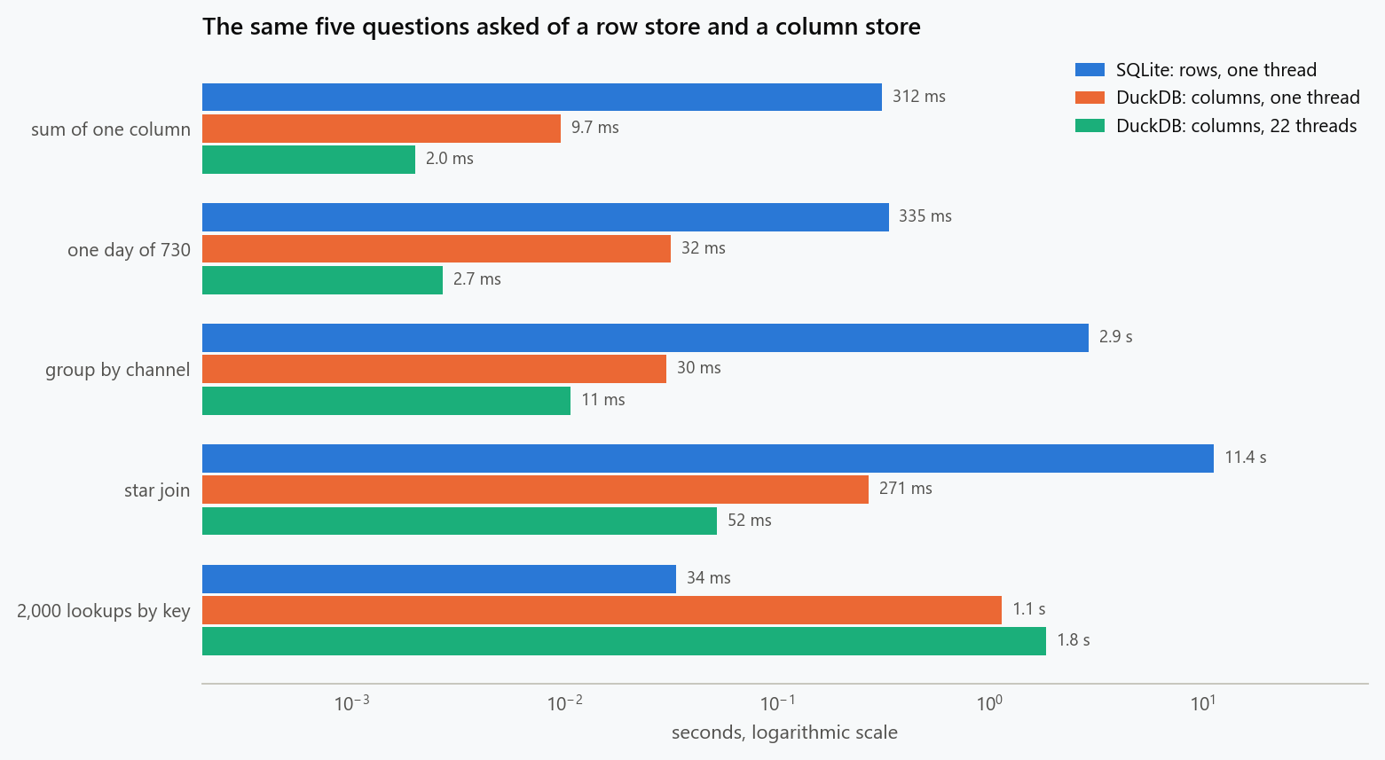
On the four analytical queries the column store wins by a factor of 11 to 97 with a single thread, and by 120 to 270 with all of them. The single-thread column is the fair comparison of layouts, and it says that most of the advantage is the layout: parallelism adds another factor of three to twelve on top. The group-by is the most lopsided because it touches two of eight columns and one of them, channel, has four distinct values, which a column store holds as a short dictionary and a row store holds five million times as text.
The last row reverses everything. Fetching 2,000 complete orders by key takes SQLite 34 milliseconds, 17 microseconds each. DuckDB takes more than a second, 570 microseconds each, although it too has an index on the key, and adding threads makes it slower. Part of that is reassembling a row from eight columns. About half is fixed cost: a DuckDB statement that does nothing at all takes 261 microseconds on this machine, against 2 in SQLite, because it is built to plan carefully for queries that run for seconds. An engine designed for throughput is a poor fit for a workload of many tiny statements, and a web application makes nothing else.
Storage follows the same logic. The orders take 195 MB in SQLite, 191 MB as CSV, 91 MB in DuckDB and 50 MB as a compressed Parquet file, which is a columnar file format and the subject of the next article. Columns of one type with few distinct values compress by a factor of four without anyone asking.
What an Index Buys
An index is a second, smaller B-tree, sorted by the indexed field, whose entries point at the rows. It lets the engine find the rows for one day without reading the rows for the other 729. SQLite will say what it intends to do if asked with EXPLAIN QUERY PLAN, and the habit of asking is worth more than any rule about indexes.
1
2
EXPLAIN QUERY PLAN
SELECT count(*), sum(amount) FROM orders WHERE order_day = 365;
1
2
3
no index                      SCAN orders                                                      335 ms
index on (order_day)          SEARCH orders USING INDEX idx_orders_day (order_day=?)           118 ms
index on (order_day, amount)  SEARCH orders USING COVERING INDEX idx_orders_day_amount (order_day=?)   0.6 ms
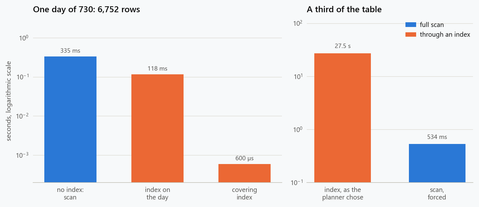
The day matches 6,752 of five million rows. With no index the engine scans the table. With an index on the day it finds the 6,752 entries at once, and then has to fetch each row from the table to read its amount: 6,752 separate walks down the main tree, which is why the gain is only a factor of three. The third index contains the amount as well, so the answer is computed from the index alone and the table is never touched. That is a covering index, and it takes the query from 335 milliseconds to 0.6, a factor of 559. It is the same idea as a column store, applied to two columns by hand.
What an Index Costs
The first cost is space and write speed. The two indexes above take the file from 195 MB to 349 MB, because an index on five million rows is itself five million entries. Each inserted row now updates three trees, and the entries of the secondary ones arrive in random order, scattered across their pages. Inserting 200,000 more orders takes 0.47 seconds into the bare table and 21.5 seconds with the two indexes in place, 46 times longer. This is why bulk loads drop their indexes first and rebuild them afterwards, which took 7.8 seconds per index here.
The second cost is subtler, and it is on the right of the figure. Ask for the orders of the first 243 days, a third of the table, summing a column the index does not contain.
1
SELECT count(*), sum(quantity) FROM orders WHERE order_day < 243;
1
2
plan chosen    SEARCH orders USING INDEX idx_orders_day_amount (order_day<?)    27.5 s
forced scan    SCAN orders    (FROM orders NOT INDEXED)                          0.53 s
The planner chose the index, with fresh statistics from ANALYZE, and the query took 27.5 seconds. Forbidden the index, it took half a second. The arithmetic was already in the first table: an index entry that does not cover the query costs one lookup in the main tree, a lookup costs 16.8 microseconds, and a third of five million rows is 1.67 million lookups, or 28.0 seconds against the 27.5 measured. The same sum explains the modest gain in the previous section: 6,752 lookups come to 113 milliseconds, and the query took 118. A scan reads the rows in the order they are stored, at about a hundred nanoseconds each.
Those two unit costs give the break-even directly. A lookup costs 16.8 microseconds per matching row and a scan 0.107 microseconds per row of the table, so the index wins only when the filter keeps less than 0.64% of the rows. Intuition says a half, and folklore says a few percent; on this table it is well under one. Planners that keep histograms of each column estimate that fraction and switch to a scan when it is large, which is the design Selinger and colleagues described in 1979 and the one PostgreSQL follows. SQLite's planner is deliberately simpler and took the index here. Whatever the engine, the defence is the same: read the plan, and time the query both ways when the filter is broad.
Transactions Are a Performance Feature
A transaction is usually introduced as a correctness device: a group of changes that happen completely or not at all, and that survive a power cut once committed, the properties Härder and Reuter (1983) named ACID. Durability has a price, because committing means waiting until the storage device confirms that the bytes are safe, and that wait is milliseconds however small the change. How often it is paid is the programmer's choice.
1
2
3
4
5
6
for row in rows:                       # 2,000 rows
    con.execute("INSERT INTO t VALUES (?, ?, ?)", row)
    con.commit()                       # one durable write per row: 25.4 s

with con:                              # one transaction, one durable write: 0.017 s
    con.executemany("INSERT INTO t VALUES (?, ?, ?)", rows)
The first loop took 25.4 seconds and the second 17 milliseconds, a factor of 1,462, for the same 2,000 rows in the same file with the same guarantee at the end. Libraries that commit after every statement by default turn this into the most common reason a load that should take a minute takes a night. The remedy is to make the transaction the unit of work: a batch of a few thousand rows, a file, a day of data. It is also the unit of recovery, since a failed batch leaves nothing half-written to clean up.
Normalise to Write, Denormalise to Read
The schema has the same two audiences. For the application that records orders, the customer's country belongs in one place, the customer table, so that changing it is one update and no two rows can disagree. That is normalisation, and its purpose is to make inconsistent states unrepresentable.
For analysis the convenient shape is a star: one long fact table with a row per event at a declared grain, here one row per order line, holding the measurements and the keys, surrounded by short dimension tables that describe customers, products and dates (Kimball and Ross, 2013). Almost every analytical question is then the same query, the one timed above: filter and group by attributes of the dimensions, aggregate measurements from the facts. The star keeps the big table narrow and numeric, which is what a column store is best at, and it gives each business concept one table with one definition, which does more for the consistency of reports than any tool.
Two habits from that literature save a great deal of later pain. State the grain of every fact table in a sentence before creating it, because most wrong totals come from joining tables of different grain. And decide what happens when a dimension changes: if a customer moves country, either past orders move with them or they do not, and the schema has to say which. Keeping the old row and adding a new one with validity dates preserves history; overwriting rewrites it. Both are legitimate, and only one of them is what the person asking the question had in mind.
What to Build
The measurements turn into a short set of decisions. Data that an application reads and writes one record at a time belongs in a row store, with an index for each selective access path and transactions around each unit of work. Data that is analysed belongs in a column store or in columnar files, loaded in batches, with a star schema whose grain is written down. When the same data serves both, which is the usual case, the answer is two copies and a scheduled transfer between them, not one database asked to be good at everything. A nightly export to Parquet that DuckDB reads directly is a complete analytical platform for far more data than most projects have.
Within either engine the working method is the one used here. Look at the plan before adding an index. Add covering indexes for the few queries that matter, and count what they cost on write. Distrust an index on a filter that keeps more than a few percent of the rows. Wrap loads in transactions, and drop indexes before bulk loads. None of it requires a database administrator, and all of it can be checked with a stopwatch.
The benchmark behind every number above is scripts/benchmarks/database_benchmarks.py in the blog-reproducibility repository, with its recorded results beside it under data/engineering/. It runs in about five minutes on a laptop. The absolute times will differ on another machine and the ratios will not differ much, which is the reason to trust them.
References
- Abadi, D. J., Madden, S. R., & Hachem, N. (2008). Column-stores vs. row-stores: how different are they really? Proceedings of the 2008 ACM SIGMOD International Conference on Management of Data, 967-980.
- Bayer, R., & McCreight, E. (1972). Organization and maintenance of large ordered indexes. Acta Informatica, 1(3), 173-189.
- Boncz, P., Zukowski, M., & Nes, N. (2005). MonetDB/X100: hyper-pipelining query execution. Proceedings of the Second Biennial Conference on Innovative Data Systems Research (CIDR), 225-237.
- Codd, E. F. (1970). A relational model of data for large shared data banks. Communications of the ACM, 13(6), 377-387.
- Härder, T., & Reuter, A. (1983). Principles of transaction-oriented database recovery. ACM Computing Surveys, 15(4), 287-317.
- Kimball, R., & Ross, M. (2013). The Data Warehouse Toolkit: The Definitive Guide to Dimensional Modeling (3rd ed.). Wiley.
- Kleppmann, M. (2017). Designing Data-Intensive Applications. O'Reilly.
- Raasveldt, M., & Mühleisen, H. (2019). DuckDB: an embeddable analytical database. Proceedings of the 2019 International Conference on Management of Data (SIGMOD), 1981-1984.
- Selinger, P. G., Astrahan, M. M., Chamberlin, D. D., Lorie, R. A., & Price, T. G. (1979). Access path selection in a relational database management system. Proceedings of the 1979 ACM SIGMOD International Conference on Management of Data, 23-34.
Embed interactive plots, widgets, and demos using <figure>, <iframe>, or <div class="interactive-embed"> containers. Ensure each embed includes descriptive captions for accessibility.
How to cite
Use the quick export buttons to save citations for reference managers or copy the formatted text directly.
Diogo Ribeiro (2026). A Database for Analysis: Rows, Columns, Indexes and the Planner. Faculty of Media Arts and Design, Technical University of Porto. https://diogoribeiro7.github.io/data-science/a_database_for_analysis_rows_columns_indexes/.


