Topics
A before-and-after testimonial presents a compact causal narrative: a person had a problem, adopted an intervention, and subsequently improved. The intervention may be a supplement, a training programme, a sleep routine, or a device that promises to optimise an unfamiliar score. Two measurements, accompanied by an account of personal experience, appear to connect the intervention to its result. There need be no fabricated screenshot or dishonest participant for this narrative to be persuasive. The measurements may be accurate, the improvement substantial, and the account sincere. What remains unresolved is how much of that improvement was caused by the intervention, because the same person might also have improved without it.
This distinction becomes consequential when the first measurement was taken at an unusual moment. Someone may start tracking sleep after an exceptionally poor week, seek a programme after a disappointing performance, or purchase a product when a monitored score crosses an alarming threshold. In each case, the starting observation has helped determine when action occurs. The resulting comparison therefore concerns a selected beginning followed by a later observation, rather than two interchangeable moments sampled from an otherwise stable process. A data analysis that ignores this selection can assign an intervention credit for a change that the selection procedure itself makes probable. The relevant scientific question is how much change should have been expected under the same recruitment and measurement rules, with the intervention absent.
The following example develops that question quantitatively. Its score, population, and intervention effects are invented; no number should be interpreted as a measurement of a real product or a clinical outcome. The purpose of the construction is to establish a possibility with explicit assumptions, then identify the additional observations needed to distinguish competing explanations. This approach also sets a limit on the criticism: demonstrating that a testimonial could arise without an effect does not establish that its particular intervention is ineffective. It establishes that the testimonial alone may be insufficient to decide.
The starting measurement is part of the selection process
Suppose a score is measured twice, with lower values regarded as preferable. Write the first measurement as $Y_0$ and the later measurement as $Y_1$. A simple model separates a person's persistent component, $\theta$, from variation specific to each occasion:
Assume that $\theta$ follows a normal distribution with mean 50 and standard deviation 8, while each $\varepsilon_t$ follows a normal distribution with mean zero and standard deviation 6. The two occasion-specific terms are independent of each other and of $\theta$; people are also independent. Nothing in this model changes between visits, and there is no intervention effect. The temporary terms can represent fluctuations in the quantity being measured as well as instrument error. Describing them as noise means that they are not persistent in this model, rather than that the participant's experience was unreal. A transient disruption can be real without being a permanent characteristic.
Each observed score has variance $8^2+6^2=100$, so its standard deviation is 10. The covariance between the two measurements is 64, because the persistent component is shared and the temporary terms are independent. Consequently, the correlation between baseline and follow-up is $\rho=64/100=0.64$. The model describes a population in which individual differences persist, but a single observation also contains substantial variation that does not persist. A correlation of 0.64 is an assumption chosen to make the arithmetic transparent. It is neither a general reliability estimate for wearable devices nor an empirical description of symptoms, laboratory measurements, or athletic performance.
Now suppose a programme recruits people whose baseline score is at least 65. Recruitment depends on the sum of two components, although only their sum is observed. People can qualify because their persistent component is high, their temporary component is high, or both. Within the recruited group, the temporary component at baseline will have a positive average: an unusually unfavourable occasion helped some people cross the threshold. The independent temporary component at follow-up has no corresponding reason to have a positive average. This asymmetry is sufficient to produce an expected reduction even though the underlying population and every person's persistent component remain unchanged. The selection problem is developed in the methodological treatment by Barnett, van der Pols, and Dobson.
Deriving the expected follow-up
The model provides a precise answer for someone observed at a particular baseline value. Because $Y_0$ and $Y_1$ are jointly normal, their conditional expectation is linear. Substituting the covariance and variance gives
At a baseline of 70, the expected follow-up is therefore 62.8. The expected fall of 7.2 points arises without assigning any action a biological, behavioural, or technical effect. It is the difference between an observation selected for being high and a prediction that accounts for the fact that some of its extremeness was temporary. The expected follow-up remains above 50 because the high baseline also supplies evidence that the persistent component is high. Regression to the mean does not imply that all participants become average, and it does not mean that persistent differences disappear. It means that a prediction based on an imperfectly persistent observation is less extreme than treating the entire observation as permanent would suggest.
An expectation is also different from an individual forecast with certainty. In this model, the conditional variance of follow-up is $100(1-0.64^2)=59.04$, giving a conditional standard deviation of approximately 7.68. For a baseline of 70, a central 95% prediction interval runs from approximately 47.74 to 77.86. Some individuals therefore worsen at the next measurement even though the conditional mean is lower. This interval describes variation in a future score under known, stipulated model parameters; it is not a confidence interval for a treatment effect. In an empirical application, uncertainty about the parameters and the adequacy of the model would require additional consideration.
The linear expression depends on the assumptions just stated. For a jointly normal pair with unequal means and standard deviations, its general form is $\mu_1+\rho(\sigma_1/\sigma_0)(y-\mu_0)$. Correlation alone does not establish a linear conditional expectation for an arbitrary pair of variables. Seasonal trends, changing measurement scales, persistent temporary disturbances, and a genuinely changing underlying state can all alter the expected trajectory. The value of the simple construction is that it isolates one mechanism, making its consequences calculable before more complex mechanisms are introduced.
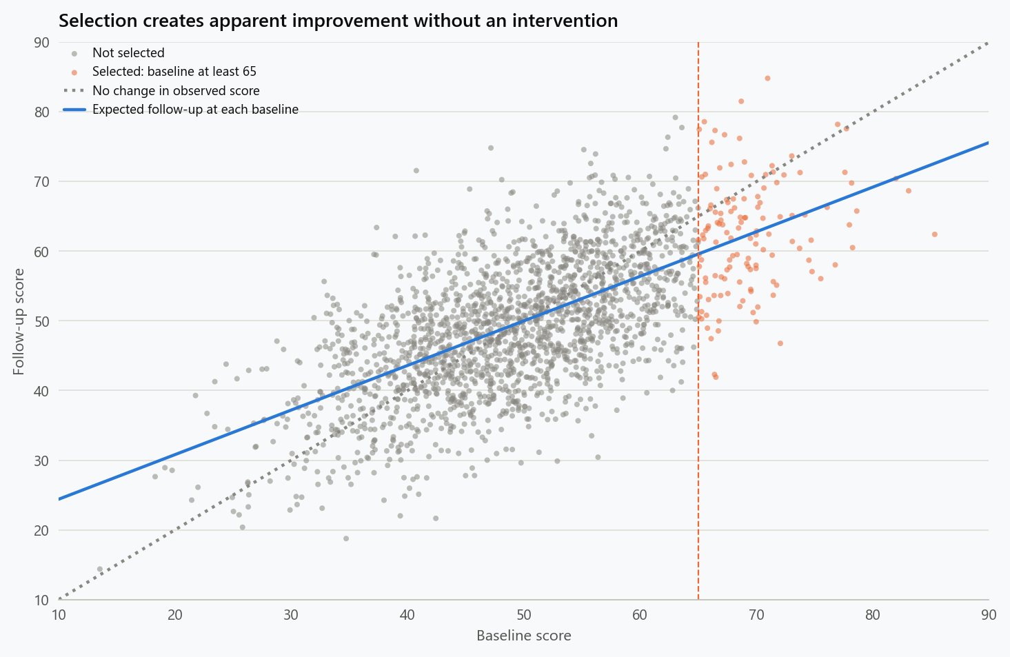
Original simulation from the stated model, with no intervention and seed 20260919. The solid line is the theoretical conditional mean; the dotted line represents an unchanged observed score. The plot illustrates individual variation, while the calculations below use exact population expectations.
From an individual baseline to a recruited cohort
An actual programme is more likely to report a group average than the conditional expectation at exactly 70. We therefore need to average over all qualifying baselines. Standardising the threshold gives $a=(65-50)/10=1.5$. Let $\phi$ and $\Phi$ denote the density and cumulative distribution functions of a standard normal variable. The proportion of the source population that qualifies is $1-\Phi(1.5)$, approximately 6.68%, and the mean of a normal distribution above a threshold is
The ratio in this expression is not an empirical adjustment fitted to secure a preferred result. It follows from integrating the upper tail: for a standard normal variable, the integral of $z\phi(z)$ from $a$ to infinity equals $\phi(a)$, and division by the tail probability produces the conditional mean. Applying the earlier follow-up formula and then averaging over the selected baselines gives $50+0.64(69.3868-50)$, approximately 62.4075. A programme that merely recruits according to this rule and measures again can therefore report an expected reduction of approximately 6.98 points. No treatment effect has been included anywhere in the calculation.
| Quantity in the synthetic population | Exact-model value, rounded |
|---|---|
| Mean score in the source population at either occasion | 50.00 |
| Proportion qualifying at baseline | 6.68% |
| Mean baseline among qualifying people | 69.39 |
| Expected follow-up among those same people | 62.41 |
| Expected follow-up minus baseline | −6.98 |
The phrase “those same people” matters. This calculation does not replace high-scoring participants with different, lower-scoring participants, and it does not depend on anyone dropping out. Everyone selected at baseline remains in the follow-up calculation. Attrition could introduce additional bias, but it is unnecessary for this effect. Nor does the programme need to choose its threshold dishonestly: recruiting people with an elevated score may be entirely reasonable for its practical purpose. The inferential error occurs when the expected consequences of that recruitment rule are attributed to an intervention without a suitable comparison.
The selected group also remains different from the source population. Its expected follow-up is 62.41 rather than 50, reflecting the persistent differences that contributed to recruitment. Calling the entire initial elevation “measurement error” would therefore be incorrect. In the construction, baseline selection identifies a mixture of persistent elevation and temporary elevation, and the mathematics estimates their contributions under the model. In real data, separating those components requires information beyond the single unusually high observation. The distinction is central to the examples discussed by Bland and Altman, and to the separate article on regression to the mean in operational analytics.
Why a small p-value cannot identify the cause
A large uncontrolled sample does not remove this problem. Under the constructed model, the selected population's mean change really is approximately −6.98. As more independently selected participants are observed, the sample mean change estimates that quantity more precisely. The variance of an individual's change within the selected population is approximately 60.98, so the standard error of the average change among 100 independent participants is approximately $\sqrt{60.98/100}=0.781$. A sample mean near its expectation would therefore sit almost nine estimated standard errors below zero. It would be unsurprising for a conventional test of zero mean change to produce a small p-value.
That statistical finding would not contradict the fact that the intervention effect is zero. The test asks whether the selected population has zero average change, and this particular population does not. The causal question asks whether follow-up differs from what it would have been under an alternative intervention condition. Those are different quantities. Increasing sample size improves estimation of the first without automatically supplying the missing comparison required for the second. This is an identification problem rather than a shortage of statistical power: the source of the change cannot be recovered merely by measuring the same uncontrolled contrast more accurately.
There is a related trap in claims that the programme “works best for people who need it most.” Define change as $D=Y_1-Y_0$. In the unselected population of this model,
The negative association means that higher baselines tend to accompany larger reductions, even though nobody receives an effective intervention. Part of the relationship is built into using the baseline on both sides of the comparison: once as a predictor and once with a minus sign in the change score. Within the selected group, the conditional expected change is still $-0.36(y-50)$, so the same qualitative pattern remains. A baseline-by-improvement plot can describe an interesting feature of the data, but it cannot establish that the causal effect is larger for initially worse-off participants. That claim requires a comparison of intervention effects across baseline levels, with the design and analysis capable of distinguishing effect variation from the statistical consequences of the baseline itself.
Improvement can coexist with benefit, no effect, or harm
To introduce an intervention, retain the same selected participants and add a constant effect $\delta$ to their follow-up score. The sign convention is important: because lower scores are preferable, a negative $\delta$ represents benefit and a positive $\delta$ represents harm relative to receiving no intervention. The expected before-and-after change becomes
The resulting comparison is more informative than a generic statement that correlation does not imply causation. It shows that the sign of the observed change need not even match the sign of the causal effect. An intervention that adds three points to follow-up makes people worse off than they would otherwise have been, yet their expected follow-up still lies below their unusually high baseline. A genuine measured improvement therefore does not, by itself, exclude harm relative to the relevant alternative. Conversely, an effective intervention can deserve some credit without deserving credit for the entire improvement.
| Hypothetical intervention condition | Expected baseline | Expected follow-up | Follow-up minus baseline | Effect relative to no intervention |
|---|---|---|---|---|
| Beneficial, $\delta=-3$ | 69.39 | 59.41 | −9.98 | −3.00 |
| No effect, $\delta=0$ | 69.39 | 62.41 | −6.98 | 0.00 |
| Harmful, $\delta=+3$ | 69.39 | 65.41 | −3.98 | +3.00 |
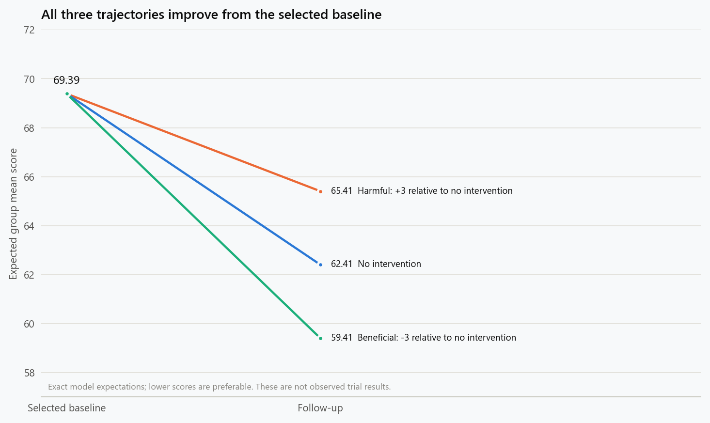
These are expectations under three stipulated conditions, rather than observed trial results. The causal comparison is the difference between follow-up conditions. Their common selected baseline makes a decrease possible in all three.
Potential-outcome notation makes the comparison explicit. Let $Y_1(1)$ be a person's follow-up under the intervention and $Y_1(0)$ the follow-up under the specified alternative. Their causal effect is $Y_1(1)-Y_1(0)$, whereas their recorded before-and-after change is $Y_1(1)-Y_0$. The baseline belongs to an earlier occasion and cannot simply substitute for the unobserved alternative at follow-up. In the additive example, the causal difference equals $\delta$ by construction. In practice, a person supplies only the outcome under the condition they actually experience, so estimating average effects requires a design that makes outcomes under different conditions meaningfully comparable.
A randomised comparison after the same eligibility assessment supplies that design under appropriate conditions. In expectation over random assignment, both groups share the selection-induced trajectory, while the intervention group additionally experiences its intervention effect. With complete, comparable follow-up, subtracting their mean changes recovers $\delta$ in this model; subtracting their follow-up means does so as well. Neither comparison is required to show zero improvement in the control group. The control group's improvement is part of the evidence needed to interpret the intervention group's improvement. Finite samples will not have exactly identical baselines or outcomes, and estimates require uncertainty intervals rather than the exact equalities in the illustrative table.
Baseline adjustment can improve precision when the analysis is appropriate to the design. Vickers and Altman discuss analysing follow-up with treatment assignment and baseline as predictors, with the analysis specified in advance. This does not mean that a change-score comparison between randomised groups is inherently biased: in the construction above, its expectation is correct. It means that validity and efficiency are separate questions, and baseline information can be used more effectively than forcing its coefficient to equal one. An uncontrolled regression cannot create a missing comparison group, while a nonrandom comparison additionally needs justification for differences in who receives each intervention. The identity of the control condition also determines the effect being estimated: an added product versus the same support without that product is a different comparison from a complete programme versus no programme.
Selecting testimonials introduces a second filter
Baseline selection is only one way a collection of accurate observations can become misleading. A publisher can also choose which outcomes to show after follow-up. To isolate this second mechanism, temporarily return to the unselected source population: no one is recruited for a high baseline, no intervention has an effect, and everyone is measured at two fixed occasions. The difference $D=Y_1-Y_0=\varepsilon_1-\varepsilon_0$ is normally distributed with mean zero and variance $36+36=72$. Some people improve substantially and others worsen substantially even though the population has no average change.
Under these assumptions, the probability of a fall of at least ten points is approximately 11.93%. Among 20 independent people, the probability that at least one supplies such a fall is
A curator could therefore find at least one apparently impressive improvement in approximately 92.1% of repeated collections of 20 people generated by this particular model. This is a probability about the availability of a testimonial, not a probability that an intervention works. The calculation neither estimates the prevalence of deceptive advertising nor describes a real platform's recommendation algorithm. It shows why the denominator matters: a striking selected case can be common among many opportunities even when the corresponding causal effect is absent. For correlated cases, different score variability, or a different definition of impressive improvement, the numerical result changes.
Combining baseline selection with outcome selection creates further distortion. A displayed case may have entered the programme after an unusually bad observation and been chosen for publication after an unusually good outcome. Unchanged and worsening cases may remain unseen, whether because of editorial choice, differential willingness to report, or loss to follow-up. Counting many displayed testimonials does not recover the missing denominator if the process that generated the display remains unknown. A prospective cohort with a defined entry rule, a fixed follow-up time, and outcomes reported for everyone answers a more interpretable descriptive question; a suitable intervention comparison is still needed for causal attribution. Scientific criticism should therefore examine the construction of the visible sample before treating its emotional vividness or numerical precision as evidence of representativeness.
What repeated baselines improve, and what they leave unresolved
Repeated measurement offers a useful response to an unstable starting value, provided the measurement schedule is specified before the results are inspected. Suppose baseline is now the average of $k$ independent occasion-specific measurements for each person. Under the same stable-component model, its variance is $64+36/k$, and the coefficient predicting a single later measurement from that average is
As $k$ grows, the average baseline contains less temporary variation and the predictive coefficient approaches one. Notice that $b_k$ is a regression coefficient; when baseline is averaged but follow-up is a single observation, their variances differ, so the coefficient should not be called their correlation. If recruitment still requires an average baseline of at least 65, the exact expected changes are as follows. Each row describes recruitment using that row's baseline rule, not repeated analyses of an identical recruited cohort.
| Measurements averaged for eligibility | Coefficient $b_k$ | Proportion qualifying | Expected baseline | Expected follow-up | Expected reduction with no intervention |
|---|---|---|---|---|---|
| 1 | 0.640 | 6.68% | 69.39 | 62.41 | 6.98 |
| 4 | 0.877 | 3.96% | 68.44 | 66.17 | 2.27 |
| 16 | 0.966 | 3.27% | 68.19 | 67.57 | 0.62 |
The reduction in apparent improvement follows from a more stable recruitment measurement, but the changing fraction admitted is equally informative. Holding the numerical threshold fixed while reducing temporary variation changes who qualifies. A comparison between studies using different screening procedures therefore cannot assume that their participants represent the same population merely because their eligibility threshold has the same printed value. The table also shows why averaging several readings after recruitment is different from using their average to determine recruitment: if selection was already triggered by one extreme measurement, replacing only the later measurement does not undo the original selection event.
The independence assumption is consequential. For occasion-specific errors with common pairwise correlation $r$, the variance of their average is $36[1+(k-1)r]/k$, rather than $36/k$. Closely spaced readings can therefore provide less new information than their count suggests. A persistent calibration error is not removed simply by collecting more readings from the same instrument, and a systematic time trend cannot be treated as independent temporary variation. The appropriate schedule depends on the scientific process, the timescale of variation, and the question being asked. Repeated baselines can make the initial state better characterised; they do not, by themselves, separate an intervention effect from recovery, concurrent behaviour changes, expectations, or other events occurring during follow-up.
Evaluating the claim without dismissing the experience
The first task when reading a testimonial is to reconstruct how its starting point was chosen. A baseline collected on a fixed calendar date in a prospectively defined population differs from the worst value someone remembers, the first alert that prompted a purchase, or the most unfavourable week available in an app. These are distinct sampling procedures, and they support distinct comparisons. The same scrutiny belongs at follow-up: a scheduled measurement differs from the best subsequent value, and a complete cohort differs from a gallery of successful cases. The scientific object is the process that generated the observations, including the observations available for selection but absent from the presentation.
The next task is to identify the outcome and the alternative condition. A device score may be reproducible without being a validated measure of the benefit being claimed. A laboratory change may have a different interpretation from improved function, reduced symptoms, or a meaningful long-term outcome. Even when the outcome is appropriate, an account of what happened after an intervention does not specify what would have happened with another intervention, ordinary care, or no additional action. A strong evaluation makes that comparison explicit and explains why the groups, measurement conditions, and follow-up procedures permit it. Random assignment supports comparability at assignment; outcome-dependent dropout, changed measurement procedures, and selective reporting can still compromise what is eventually analysed.
Regression to the mean also should not become a universal explanation deployed without evidence. Its magnitude depends on the population, selection rule, temporal structure, and measurement properties. A person who improves may have benefited from an effective intervention, experienced a spontaneous change, changed several behaviours simultaneously, or encountered a combination of these mechanisms. The model developed here does not allocate credit among those possibilities in any actual testimonial. It demonstrates why that allocation cannot be read directly from two values. In particular, an observed reduction does not prove efficacy, and the possibility of regression does not prove inefficacy; both conclusions would exceed the information supplied.
The appropriate standard of science communication is therefore to preserve the distinction between an experience and the causal claim attached to it. An experience can motivate research, identify outcomes that matter to participants, and reveal practical details that an aggregate result might overlook. Estimating an intervention's contribution requires a further argument about selection, measurement, and the relevant alternative trajectory. In the worked example, every condition produced improvement from baseline, while their effects ranged from benefit to harm. That is why the defensible question is how the outcome compares with what would otherwise have occurred, and why answering it requires more than the visible distance between “before” and “after.”
Reproducing the calculations
The calculation and figure script prints the exact cohort moments, prediction interval, testimonial-selection probabilities, and repeated-baseline results. Running the command below from the reproducibility repository performs those calculations using the Python standard library without writing files. Running it without that option also regenerates the two figures using Matplotlib and the site's chart style. The first figure uses 2,000 simulated people; its empirical averages need not equal the population expectations reported in the tables. Separate tests check the threshold calculations against numerical integration, compare the change moments with a latent-variable simulation, and verify the effect contrasts and limiting cases. None of these computational checks establishes that the synthetic model fits a particular product, person, or dataset.
1
poetry run python scripts/figures/statistics/testimonial_selection.py --dry-run
References
- Barnett, A. G., van der Pols, J. C., and Dobson, A. J. (2005). Regression to the mean: what it is and how to deal with it. International Journal of Epidemiology, 34(1), 215–220.
- Bland, J. M., and Altman, D. G. (1994). Some examples of regression towards the mean. BMJ, 309, 780.
- Vickers, A. J., and Altman, D. G. (2001). Analysing controlled trials with baseline and follow up measurements. BMJ, 323, 1123–1124.
Embed interactive plots, widgets, and demos using <figure>, <iframe>, or <div class="interactive-embed"> containers. Ensure each embed includes descriptive captions for accessibility.
How to cite
Use the quick export buttons to save citations for reference managers or copy the formatted text directly.
Diogo Ribeiro (2026). What a Before-and-After Testimonial Can Establish. Faculty of Media Arts and Design, Technical University of Porto. https://diogoribeiro7.github.io/science-communication/what_before_and_after_testimonials_can_establish/.


