Topics
A numerical solver returns a smooth trajectory. The state stays nonnegative. Total mass is conserved to floating-point precision. Halving the time step makes successive solutions agree at approximately second order.
That sounds reassuring. In the example below, all of those observations are compatible with solving the wrong differential equation.
Before optimizing a numerical kernel, we need independent evidence that it computes the mathematical object we intended. Timing an unverified calculation can tell us how quickly it produces numbers. It does not establish what those numbers approximate.
Start with a mathematical contract
Consider a closed system in which a quantity moves from state $x$ to state $y$:
Time and state units are scaled for this example. There is no empirical claim that this model describes a particular chemical or physical process.
We can derive three independent properties before implementing a solver. First,
Second, the total is conserved because the derivatives cancel:
Third, both states lie between zero and one for $t\ge0$.
These properties check different things. Conservation constrains the sum. Nonnegativity constrains the permitted region. The analytic solution checks the location within that region at each time. No one of them subsumes the others.
Implement two explicit methods
Write the state vector as $z=(x,y)$ and its derivative as $f(z)$. Forward Euler uses
Heun's method first makes an Euler prediction, then averages the derivative at the original and predicted states:
For this smooth problem over a fixed interval, with sufficiently small stable steps and negligible roundoff, we expect first-order global error from Euler and second-order error from Heun.
The implementation below integrates to exactly $t=1$ using an integer number of equal steps. It also records the largest mass discrepancy along the computed path.
1
2
3
4
5
6
7
8
9
10
11
12
13
14
15
16
17
18
19
20
21
22
23
24
25
26
27
28
29
30
31
32
33
from math import exp, log2
import numpy as np

def solve(steps, method="heun", rate=2.0):
    if not isinstance(steps, (int, np.integer)) or steps < 1:
        raise ValueError("steps must be a positive integer")
    if method not in {"euler", "heun"}:
        raise ValueError("unknown method")
    h = 1 / steps
    z = np.array([1.0, 0.0])
    mass_error = 0.0

    def rhs(state):
        return rate * state[0] * np.array([-1.0, 1.0])

    for _ in range(steps):
        k1 = rhs(z)
        if method == "euler":
            z = z + h * k1
        else:
            z = z + h * (k1 + rhs(z + h * k1)) / 2
        mass_error = max(mass_error, abs(z.sum() - 1))
    return z, mass_error

exact = np.array([exp(-2), 1 - exp(-2)])
for method in ("euler", "heun"):
    previous = None
    for steps in (5, 10, 20, 40, 80):
        endpoint, mass_error = solve(steps, method)
        error = float(np.max(np.abs(endpoint - exact)))
        order = None if previous is None else log2(previous / error)
        print(method, steps, error, mass_error, order)
        previous = error
The rate argument will let us inject a controlled fault. It is set to the required value 2 for the initial comparison.
Measure error under refinement
Define the endpoint error against the independently derived solution:
If the dominant error is $Ch^p$, halving $h$ gives the observed order
The run gives the following values; each order compares that row with the preceding coarser step.
| Steps | $h$ | Euler error | Euler order | Heun error | Heun order |
|---|---|---|---|---|---|
| 5 | 0.2000 | 0.0575753 | — | 0.0100581 | — |
| 10 | 0.1000 | 0.0279611 | 1.042 | 0.00211275 | 2.251 |
| 20 | 0.0500 | 0.0137586 | 1.023 | 0.000487174 | 2.117 |
| 40 | 0.0250 | 0.00682313 | 1.012 | 0.000117144 | 2.056 |
| 80 | 0.0125 | 0.00339748 | 1.006 | 0.0000287318 | 2.028 |
The orders approach the expected values as the step decreases. We do not require the coarsest pair to give exactly one or two: higher-order terms still contribute there.
All these runs conserve mass with maximum discrepancy below $5\times10^{-16}$. The first-order method and the more accurate second-order method therefore look equally good under the conservation check, despite different solution errors.
Refinement studies require an asymptotic regime in which the leading error term dominates. The same principle underlies spatial grid-convergence assessment; the particular table here concerns time-step refinement in an ODE. NASA NPARC, Examining Spatial Grid Convergence.
Inject a fault that the invariant cannot detect
Now replace the intended coefficient 2 with 1.8 in both derivatives. The numerical method is unchanged, but the implemented model becomes
Its mass still sums to one. Its exact states are still nonnegative. Heun still converges at second order to the solution of the equation it is given.
The limiting value is simply wrong for the original contract:
The endpoint error against the intended solution approaches
| Steps | Wrong-rate Heun error against intended solution | Maximum mass discrepancy |
|---|---|---|
| 5 | 0.0385767 | $2.22\times10^{-16}$ |
| 10 | 0.0318129 | 0 |
| 20 | 0.0303939 | $3.33\times10^{-16}$ |
| 40 | 0.0300675 | $2.22\times10^{-16}$ |
| 80 | 0.0299891 | $2.22\times10^{-16}$ |
The discretization error shrinks, leaving a discrepancy that further refinement does not remove. A tighter step-size tolerance cannot correct the wrong coefficient.
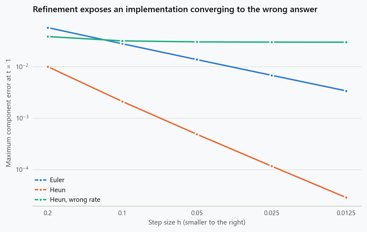
This is a deliberately injected fault in a small example, not evidence of a defect in a numerical library. Its purpose is to demonstrate what a conservation check can miss.
Self-convergence does not identify the limiting answer
When an analytic solution is unavailable, a common diagnostic compares three numerical resolutions:
The differences cancel the unknown limiting value. That is why the diagnostic can estimate order without an exact solution. It is also why it cannot establish that the limit is correct.
1
2
3
4
5
# Continue from the previous code block.
wrong = [solve(n, "heun", rate=1.8)[0][0] for n in (20, 40, 80)]
observed = log2(abs(wrong[0] - wrong[1]) / abs(wrong[1] - wrong[2]))
print(f"Self-convergence order: {observed:.3f}")
print(f"Limiting error: {exp(-1.8) - exp(-2):.7f}")
The observed self-convergence order is 2.058. An apparently successful order check coexists with the wrong limiting solution.
Self-convergence is valuable evidence about resolution dependence. It needs to be combined with evidence connecting the implementation to the intended equations: analytic cases, independently implemented references, manufactured solutions, or identities that exercise the relevant terms.
For example, a time-dependent manufactured test could specify $x(t)=\cos t$ and use the equation $x'=-2x+2\cos t-\sin t$, with $x(0)=1$. The solution is known by construction, and the forcing term exercises a part of a general ODE implementation that the autonomous conversion example does not cover.
Accuracy, stability, and physical constraints are separate checks
Conservation also does not enforce nonnegativity. One Euler step of size $h=0.75$ from the initial state gives
The total is exactly one, but the states violate the permitted range.
For the scalar decay component, Euler's amplification factor is $1-2h$. Absolute stability requires $|1-2h|<1$, or $0<h<1$. Preserving nonnegativity from a positive state requires the stronger condition $h\le0.5$.
Thus a stable calculation can violate a physical constraint, and a constraint-preserving calculation can still have an unacceptable approximation error. Each check should have an explicit purpose.
Refinement has limits too. Roundoff can dominate at sufficiently small steps; nonsmooth solutions can reduce observed order; adaptive solvers introduce internal tolerances that must be considered alongside output spacing. A convergence plot should not be interpreted beyond the regime it actually tests.
Compare work at a common accuracy requirement
A comparison at the same number of steps answers how much work each step costs. It does not necessarily compare the work required to solve the problem to an acceptable accuracy.
Suppose the requirement is endpoint error at most $10^{-4}$ under the norm defined above. Search the sequence of step counts $1,2,4,8,\ldots$ for the first acceptable run:
1
2
3
4
5
6
7
8
9
10
11
# Continue from the first code block; no timing claims are made here.
for method in ("euler", "heun"):
    steps = 1
    error = float("inf")
    while error > 1e-4:
        endpoint, _ = solve(steps, method)
        error = float(np.max(np.abs(endpoint - exact)))
        if error > 1e-4:
            steps *= 2
    evaluations = steps if method == "euler" else 2 * steps
    print(method, steps, evaluations, error)
| Method | First acceptable power-of-two step count | RHS evaluations in that run | Endpoint error |
|---|---|---|---|
| Euler | 4,096 | 4,096 | $6.61\times10^{-5}$ |
| Heun | 64 | 128 | $4.51\times10^{-5}$ |
These are counts for the accepted runs, excluding the work spent searching the grid. They are not the smallest possible integer step counts and not measured wall-clock times.
Heun uses two derivative evaluations per step, yet far fewer evaluations to satisfy this error requirement. Actual runtime also depends on implementation overhead, memory access, hardware, and the cost of the derivative. This example supports comparing methods at a common accuracy target; it does not establish a universal speed ranking.
Make verification part of the optimization workflow
A useful verification record states the equation, parameters, initial and boundary conditions, reference solution, error norm, refinement sequence, and expected behavior. Keep more than one diagnostic because their blind spots differ.
Unit tests can implement these checks. The distinction is in what they assert: a test that a function returns a finite two-element array checks an interface property; a test that refinement approaches an independently derived solution checks a numerical claim. Both can belong in the same test suite.
Before and after an optimization, compare the solution error and relevant invariants over several regimes. Include limiting parameters and cases where the method is expected to fail. If the optimization changes summation order, vectorization, precision, or solver tolerances, decide which numerical differences are acceptable in terms of the scientific quantity being computed.
Verification still does not validate the model against reality. It establishes evidence that the implementation solves the specified mathematical problem. Whether that problem represents a real system requires a separate comparison with observations and an assessment of model assumptions. NASA NPARC, Verification Assessment.
The site's article on executable mathematics develops the broader idea of testing relations between computations. Here, the essential relation is between resolution, the intended equation, and the limiting answer. Performance measurements become useful once that relation has been checked.
Run poetry run python scripts/figures/engineering/numerical_verification.py in the reproducibility repository to reproduce the tables and figure. The reproduction script uses Python, NumPy, and Matplotlib; the reported calculations used NumPy 2.3.5 and Matplotlib 3.10.8.
Embed interactive plots, widgets, and demos using <figure>, <iframe>, or <div class="interactive-embed"> containers. Ensure each embed includes descriptive captions for accessibility.
How to cite
Use the quick export buttons to save citations for reference managers or copy the formatted text directly.
Diogo Ribeiro (2026). Numerical Verification Comes Before Optimization. Faculty of Media Arts and Design, Technical University of Porto. https://diogoribeiro7.github.io/programming/numerical_verification_before_optimization/.


