Topics
A delivery-time model predicts 36 minutes for an order. It is a good model, in the sense that its predictions are unbiased, and 40 percent of deliveries arrive later than predicted. The customer did not ask for the average. They asked when the parcel would arrive, and a promise that fails four times in ten is not a promise. The number they wanted was a quantile, and a model that predicts the mean does not contain it.
The Mean Is the Wrong Summary for a Promise
Two features of real outcomes make the mean a poor basis for a commitment. The distribution is skewed, so the mean sits above the typical case and below the bad ones; and its spread depends on the inputs, so a margin that is right for one order is wrong for another.
The standard workaround is to add a fixed margin to a least-squares prediction, usually the residual standard deviation times a normal quantile. That assumes the residuals are symmetric and have the same spread everywhere, and both assumptions are wrong exactly where a promise is hardest to keep.
Quantile regression drops both. For a chosen probability $\tau$ it fits the conditional $\tau$-quantile of the outcome directly, by minimising the pinball loss
which charges $\tau$ per unit of under-prediction and $1 - \tau$ per unit of over-prediction. Minimising it over a linear function of the inputs, as Koenker and Bassett proposed, gives a linear program with one set of coefficients per quantile. Because each quantile has its own coefficients, the spread can depend on the inputs, and the shape of the distribution can change with them.
A Simulation Where the Spread Depends on Load
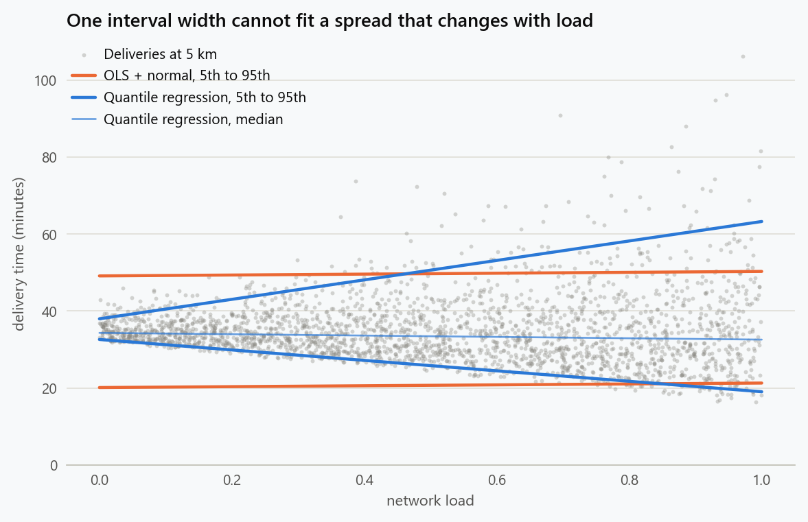
Delivery time depends on distance through the mean, and on network load through the spread. At low load a delivery takes about as long as expected; at high load it can take much longer, and the tail is one-sided.
1
2
3
4
5
6
7
8
9
10
11
12
13
14
15
16
17
18
19
20
21
22
23
24
25
26
27
28
29
30
31
32
33
34
35
import numpy as np
import statsmodels.api as sm
from scipy import stats
from sklearn.ensemble import HistGradientBoostingRegressor

rng = np.random.default_rng(0)
n = 6000
distance = rng.uniform(1, 10, n)               # km
load = rng.uniform(0, 1, n)                    # network load, 0 = quiet, 1 = saturated
mu = 20 + 3.0 * distance                       # minutes
sigma = 2 + 12 * load                          # spread rises with load
y = mu + sigma * (rng.gamma(2.0, 1.0, n) - 2.0) / np.sqrt(2.0)   # skewed, mean zero, sd sigma
X = np.column_stack([distance, load])
tr, te = np.arange(n) < 4000, np.arange(n) >= 4000

# least squares with a normal 90% interval
Xc = sm.add_constant(X)
ols = sm.OLS(y[tr], Xc[tr]).fit()
resid_sd = ols.resid.std()
pred = ols.predict(Xc[te])
ols_lo, ols_hi = pred - 1.645 * resid_sd, pred + 1.645 * resid_sd
print(f"OLS: {ols.params.round(2)}, residual sd {resid_sd:.2f}")

# linear quantile regression at the 5th, 50th and 95th percentiles
qs = (0.05, 0.5, 0.95)
qr = {q: sm.QuantReg(y[tr], Xc[tr]).fit(q=q) for q in qs}
for q in qs:
    print(f"quantile {q}: coefficients {qr[q].params.round(2)}")
qr_pred = {q: qr[q].predict(Xc[te]) for q in qs}

# gradient boosting with the pinball loss, default settings
gb = {q: HistGradientBoostingRegressor(loss="quantile", quantile=q, max_iter=300,
                                        learning_rate=0.05, random_state=0).fit(X[tr], y[tr])
      for q in qs}
gb_pred = {q: gb[q].predict(X[te]) for q in qs}
| Model | Intercept | Distance (min/km) | Load |
|---|---|---|---|
| Least squares (mean) | 19.46 | 3.03 | 1.17 |
| Quantile 0.05 | 17.50 | 3.02 | -13.60 |
| Quantile 0.50 | 19.27 | 3.01 | -1.75 |
| Quantile 0.95 | 22.53 | 3.09 | 25.32 |
Distance costs three minutes per kilometre at every quantile, which is what a shift in the centre looks like. Load is different. Least squares says it adds 1.17 minutes to the mean, which is sampling noise: load has no effect on the mean in this simulation, and 1.17 is an unlucky draw about 2.3 standard errors from zero. The quantile fits say that load lowers the fast deliveries a little and raises the slow ones a lot: a saturated network adds 25 minutes to the 95th percentile and takes 1.75 minutes off the median, because a wider right-skewed spread pulls the median further below the mean. Load does not slow deliveries. It makes them unpredictable, and that is a different operational fact with a different response.
Coverage Where It Matters
A 90 percent interval should contain 90 percent of outcomes, and it should do so for every kind of order, not on average across them.
1
2
3
4
5
6
7
8
9
10
11
12
13
14
15
16
17
def coverage(lo, hi, mask):
    return np.mean((y[te][mask] >= lo[mask]) & (y[te][mask] <= hi[mask]))

bins = [(0, 0.25), (0.25, 0.5), (0.5, 0.75), (0.75, 1.0)]
print("load        OLS+normal   linear QR   boosting QR   OLS width   QR width")
for lo, hi in bins:
    m = (load[te] >= lo) & (load[te] < hi)
    print(f"{lo:.2f}-{hi:.2f}   {coverage(ols_lo, ols_hi, m):>8.0%}   "
          f"{coverage(qr_pred[0.05], qr_pred[0.95], m):>9.0%}   "
          f"{coverage(gb_pred[0.05], gb_pred[0.95], m):>10.0%}   "
          f"{np.mean(ols_hi[m] - ols_lo[m]):>8.1f}   {np.mean(qr_pred[0.95][m] - qr_pred[0.05][m]):>7.1f}")
allm = np.ones(te.sum(), bool)
print(f"overall     {coverage(ols_lo, ols_hi, allm):>8.0%}   "
      f"{coverage(qr_pred[0.05], qr_pred[0.95], allm):>9.0%}   "
      f"{coverage(gb_pred[0.05], gb_pred[0.95], allm):>10.0%}")
print(f"OLS interval misses: {np.mean(y[te] > ols_hi):.1%} above, {np.mean(y[te] < ols_lo):.1%} below")
print(f"QR  interval misses: {np.mean(y[te] > qr_pred[0.95]):.1%} above, {np.mean(y[te] < qr_pred[0.05]):.1%} below")
| Load | Least squares, normal margin | Linear quantile regression | Boosting, default | Least-squares width | Quantile width |
|---|---|---|---|---|---|
| 0.00 to 0.25 | 99% | 87% | 80% | 29.0 | 10.1 |
| 0.25 to 0.50 | 96% | 90% | 82% | 29.0 | 20.1 |
| 0.50 to 0.75 | 93% | 88% | 80% | 29.0 | 29.8 |
| 0.75 to 1.00 | 83% | 90% | 82% | 29.0 | 39.5 |
| Overall | 93% | 89% | 81% |
The least-squares interval covers 93 percent overall, which would pass a casual check. By segment it covers 99 percent of quiet-network orders with an interval three times wider than needed, and 83 percent of saturated-network orders with an interval that is too narrow. It is wrong in both directions and right on average. The quantile interval is within a few points of 90 percent in every segment, and its width runs from 10 minutes to 40.
The misses are lopsided too. The least-squares interval is exceeded above 5.1 percent of the time and below 2.0 percent: its symmetric margin is too generous on the early side, where nobody minds, and not generous enough on the late side, where the promise fails. The quantile interval misses 5.2 percent above and 5.9 percent below, which is what a 5th-to-95th interval should do.
Pinball Loss Is the Scorecard
Coverage tells whether an interval is honest. It does not tell whether it is sharp: an interval from zero to infinity has perfect coverage. The pinball loss evaluated at each quantile rewards both, and it is the proper scoring rule for a quantile in the sense of Gneiting and Raftery: the true conditional quantile minimises its expectation, and nothing else does.
1
2
3
4
5
6
7
8
9
def pinball(q, yv, pv):
    d = yv - pv
    return np.mean(np.maximum(q * d, (q - 1) * d))

print("quantile   OLS+normal   linear QR   boosting QR")
for q in qs:
    ols_q = pred + resid_sd * stats.norm.ppf(q)
    print(f"{q:<10} {pinball(q, y[te], ols_q):>10.3f}   {pinball(q, y[te], qr_pred[q]):>9.3f}   "
          f"{pinball(q, y[te], gb_pred[q]):>11.3f}")
| Quantile | Least squares, normal margin | Linear quantile regression | Boosting, default |
|---|---|---|---|
| 0.05 | 0.739 | 0.500 | 0.568 |
| 0.50 | 3.070 | 2.950 | 3.096 |
| 0.95 | 1.257 | 1.145 | 1.233 |
The linear quantile regression wins at every quantile, by a third at the lower tail. The boosting model, which can represent any shape the data has, loses to it at every quantile as well. That is the next section.
Flexible Quantile Learners Need Watching
Gradient boosting with the quantile loss is the natural choice when the relationship is not linear, and it comes with two problems that the linear version does not have.
1
2
3
4
5
6
7
8
9
10
11
12
13
14
15
16
17
def fit_gb(q, **kw):
    return HistGradientBoostingRegressor(loss="quantile", quantile=q, random_state=0,
                                         **kw).fit(X[tr], y[tr]).predict(X[te])

configs = {
    "default (300 rounds, leaf >= 20)": dict(max_iter=300, learning_rate=0.05),
    "regularised (depth 3, leaf >= 200)": dict(max_iter=300, learning_rate=0.05,
                                                max_depth=3, min_samples_leaf=200),
}
for name, kw in configs.items():
    lo, hi = fit_gb(0.05, **kw), fit_gb(0.95, **kw)
    cov = [coverage(lo, hi, (load[te] >= a) & (load[te] < b)) for a, b in bins]
    print(f"{name}: coverage by load " + ", ".join(f"{c:.0%}" for c in cov)
          + f", overall {coverage(lo, hi, allm):.0%}")
    preds = np.array([fit_gb(q, **kw) for q in np.arange(0.1, 0.91, 0.1)])
    crossing = np.mean(np.any(np.diff(preds, axis=0) < 0, axis=0))
    print(f"   adjacent-quantile crossings (0.1 to 0.9 by 0.1): {crossing:.1%} of test points")
| Configuration | Coverage by load segment | Overall | Test points with crossing quantiles |
|---|---|---|---|
| Default: 300 rounds, at least 20 per leaf | 80%, 82%, 80%, 82% | 81% | 33.2% |
| Regularised: depth 3, at least 200 per leaf | 88%, 88%, 84%, 89% | 87% | 7.9% |
The tails are estimated from few points. The 5th percentile inside a leaf of twenty observations is the smallest one, and the model overfits the tails while looking fine in the middle. The default configuration produces an interval that claims 90 percent and delivers 81. A quantile model needs more regularisation than the same model fitted to the mean, and its coverage has to be checked on held-out data by segment, as above. Where the check fails, conformalised quantile regression, from Romano, Patterson and Candès, adjusts the interval's edges by a calibrated amount so that the coverage holds, at the cost of some sharpness.
Nothing forces the quantiles to be ordered. Each quantile is a separate model, and separately fitted models can cross: a 40th percentile above the 50th for some inputs. The default model crosses on a third of the test points across nine quantiles, the regularised one on eight percent. The simple repair is to sort the predicted quantiles for each observation, which Chernozhukov, Fernández-Val and Galichon show never makes the estimates worse. The structural repair is a model that fits the whole conditional distribution at once, such as quantile regression forests, which read all quantiles from the same leaves and therefore cannot cross.
Choosing the Quantile to Promise
Which quantile to promise is a cost question, and it has a closed form. If a late delivery costs $c_L$ and an early one $c_E$, the promise that minimises expected cost is the quantile
1
2
3
4
print(f"mean delivery time {y.mean():.1f}, median {np.median(y):.1f}")
print(f"share of deliveries later than the OLS point prediction: {np.mean(y[te] > pred):.1%}")
for c_late, c_early in ((1, 1), (4, 1), (9, 1)):
    print(f"late costs {c_late}x early: promise the {c_late / (c_late + c_early):.2f} quantile")
If late and early cost the same, promise the median, which here is 35.9 minutes against a mean of 36.6. If a late delivery costs four times an early one, promise the 80th percentile; nine times, the 90th. The least-squares prediction is a promise at about the 60th percentile, late 40 percent of the time, and it corresponds to no cost ratio anyone chose. This is the newsvendor result, and it applies wherever a number is committed to under asymmetric costs: safety stock, staffing, capacity, delivery windows, remaining useful life.
Reading the Coefficients
The coefficient table is the part of quantile regression that has no analogue in a mean model, and it is worth reading as a finding rather than as a fit. A predictor whose coefficient is the same at every quantile shifts the whole distribution: distance, here. A predictor whose coefficient rises across the quantiles widens the distribution: load. A predictor whose coefficients diverge in sign at the two tails changes the shape. In a mean model all three look like a single number, the average of the effects across all quantiles. For load that average is zero, a large rise for bad deliveries cancelling falls for fast and typical ones, and the 1.17 minutes that least squares attributes to load is noise around that zero.
That reading changes the operational response. A shift is addressed by changing the centre: a shorter route, a faster process. A widening is addressed by adding capacity at high load, or by promising a wider window at high load and a tight one at low load, which the quantile model prices exactly.
What to Do
- Ask which quantile the decision needs before fitting anything, and compute it from the costs of being early and late.
- Fit quantiles directly rather than adding a margin to a mean, whenever the spread could depend on the inputs, which is nearly always.
- Check coverage by segment, not on average. A 90 percent interval that covers 99 percent of easy cases and 83 percent of hard ones is failing.
- Score with the pinball loss at each quantile, and compare against the mean-plus-margin baseline.
- Regularise flexible quantile models harder than their mean counterparts, sort the predicted quantiles, and conformalise if coverage still falls short.
- Read the coefficient table across quantiles as a description of how the inputs move the distribution, and act on the shape, not just the centre.
The figure generator in the blog-reproducibility repository reproduces this article's figure; run it with --dry-run to print the numbers behind the figure without writing an image.
References
- Koenker, R., & Bassett, G. (1978). Regression quantiles. Econometrica, 46(1), 33-50.
- Koenker, R., & Hallock, K. F. (2001). Quantile regression. Journal of Economic Perspectives, 15(4), 143-156.
- Koenker, R. (2005). Quantile Regression. Cambridge University Press.
- Meinshausen, N. (2006). Quantile regression forests. Journal of Machine Learning Research, 7, 983-999.
- Chernozhukov, V., Fernández-Val, I., & Galichon, A. (2010). Quantile and probability curves without crossing. Econometrica, 78(3), 1093-1125.
- Romano, Y., Patterson, E., & Candès, E. (2019). Conformalized quantile regression. Advances in Neural Information Processing Systems, 32.
- Gneiting, T., & Raftery, A. E. (2007). Strictly proper scoring rules, prediction, and estimation. Journal of the American Statistical Association, 102(477), 359-378.
Embed interactive plots, widgets, and demos using <figure>, <iframe>, or <div class="interactive-embed"> containers. Ensure each embed includes descriptive captions for accessibility.
How to cite
Use the quick export buttons to save citations for reference managers or copy the formatted text directly.
Diogo Ribeiro (2026). Quantile Regression: Predicting the Range, Not the Average. Faculty of Media Arts and Design, Technical University of Porto. https://diogoribeiro7.github.io/statistics/quantile_regression_predicting_the_range/.


