Topics
An experiment finishes and reports a 4.2 percent lift, significant. The team ships it and books 4.2 percent. A year later the metric has not moved by anything like the sum of the year's wins, and everyone blames measurement.
The programme already contained the information needed to predict that. Two hundred previous experiments in the same product had true effects spread around roughly one percentage point. Against that background, a measured 4.2 percent from a test with a one-point standard error is half noise, and its honest estimate is closer to two. Nothing about this requires a philosophical commitment to Bayesian inference. The distribution of past effects is data, and ignoring it is the unusual choice.
The Spread of Real Effects Is Measurable
The estimates from a programme vary for two reasons: the true effects differ, and each is measured with error. Their variance is the sum of the two, so subtracting the average sampling variance leaves the spread of the truth.
1
2
3
4
5
6
7
8
9
10
11
12
13
14
15
16
17
18
19
20
21
22
23
24
25
26
27
28
29
30
31
32
33
34
import numpy as np

RNG = np.random.default_rng(71)
K = 200                       # experiments in the programme
TAU = 0.010                   # real effects have this spread: one percentage point
REPS = 400


def programme(k=K, tau=TAU, se_lo=0.004, se_hi=0.020, rng=RNG):
    """True effects drawn from a common distribution, each measured with its
    own precision because tests ran for different lengths."""
    truth = rng.normal(0.0, tau, k)
    se = rng.uniform(se_lo, se_hi, k)
    est = truth + rng.normal(0, se)
    return truth, est, se


def estimate_tau(est, se):
    """The spread of the estimates is the spread of the truth plus the noise."""
    return np.sqrt(max(est.var(ddof=1) - np.mean(se ** 2), 1e-12))


def shrink(est, se, tau_hat):
    b = tau_hat ** 2 / (tau_hat ** 2 + se ** 2)
    return b * est, b


truth, est, se = programme()
tau_hat = estimate_tau(est, se)
shrunk, b = shrink(est, se, tau_hat)
print(f"spread of the true effects: {TAU:.4f}, estimated from the results: {tau_hat:.4f}")
print(f"average shrinkage factor: {b.mean():.2f} (from {b.min():.2f} to {b.max():.2f})")
print(f"root mean squared error, raw estimates:    {np.sqrt(np.mean((est - truth) ** 2)):.5f}")
print(f"root mean squared error, shrunk estimates: {np.sqrt(np.mean((shrunk - truth) ** 2)):.5f}")
| Quantity | Value |
|---|---|
| True spread of effects | 0.0100 |
| Spread estimated from the results | 0.0090 |
| Average shrinkage factor | 0.40, from 0.17 to 0.83 |
| Error of the raw estimates | 0.01278 |
| Error of the shrunk estimates | 0.00689 |
Each estimate is multiplied by $\tau^2/(\tau^2 + \sigma_i^2)$, the share of its variance that is real signal. A precise experiment keeps 83 percent of its measured effect; an imprecise one keeps 17 percent. Nothing is discarded and nothing is assumed beyond the programme's own history.
1
2
3
4
5
6
7
8
9
10
11
raw_rmse, sh_rmse, taus = [], [], []
for r in range(REPS):
    truth, est, se = programme(rng=np.random.default_rng(200 + r))
    t_hat = estimate_tau(est, se)
    sh, _ = shrink(est, se, t_hat)
    raw_rmse.append(np.sqrt(np.mean((est - truth) ** 2)))
    sh_rmse.append(np.sqrt(np.mean((sh - truth) ** 2)))
    taus.append(t_hat)
print(f"estimated spread: {np.mean(taus):.4f} +- {np.std(taus):.4f}, truth {TAU:.4f}")
print(f"raw error {np.mean(raw_rmse):.5f}, shrunk error {np.mean(sh_rmse):.5f}, "
      f"reduction {1 - np.mean(sh_rmse) / np.mean(raw_rmse):.1%}")
| Quantity | Over 400 programmes |
|---|---|
| Estimated spread of true effects | 0.0098 ± 0.0014 against a truth of 0.0100 |
| Error of the raw estimates | 0.01284 |
| Error of the shrunk estimates | 0.00744 |
| Reduction | 42.1% |
The estimator of the spread is accurate, and the shrunk estimates are closer to the truth by 42 percent in root mean squared error. That improvement is not a trick of averaging: it holds programme by programme, in all 400 of them, and it is the same phenomenon that makes a batting average early in a season a poor forecast of the rest of it.
The Ones That Looked Like Wins
The averages hide where the gain comes from. It is concentrated in exactly the results a programme acts on: the positive, significant ones.
1
2
3
4
5
6
7
8
9
10
11
truth, est, se = programme(rng=np.random.default_rng(7))
t_hat = estimate_tau(est, se)
sh, b = shrink(est, se, t_hat)
win = (est > 1.96 * se)                      # positive and significant: the ones you ship
top = np.argsort(-est)[:10]
print(f"positive and significant: {win.sum()} of {K}")
print(f"  their average raw estimate    {est[win].mean():+.4f}")
print(f"  their average true effect     {truth[win].mean():+.4f}")
print(f"  their average shrunk estimate {sh[win].mean():+.4f}")
print(f"top ten by raw estimate: raw {est[top].mean():+.4f}, "
      f"truth {truth[top].mean():+.4f}, shrunk {sh[top].mean():+.4f}")
| Group | Raw estimate | True effect | Shrunk estimate |
|---|---|---|---|
| The 7 positive significant results | +0.0209 | +0.0119 | +0.0108 |
| The top ten by raw estimate | +0.0264 | +0.0085 | +0.0087 |
The top ten by measured effect average 2.64 percent and are worth 0.85. The shrunk estimate says 0.87. Ranking by a noisy measurement selects for luck as well as quality, and the shrinkage undoes almost exactly the amount of luck that the selection introduced.
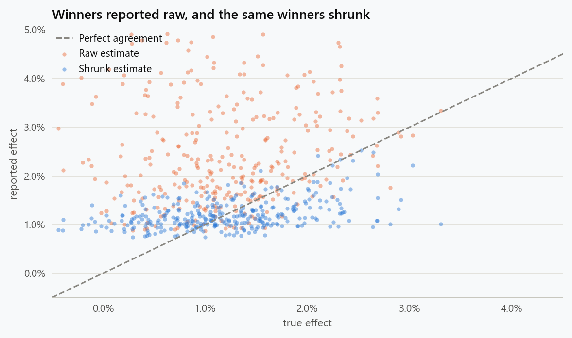
How Far They Fall Back Depends on Precision
1
2
3
4
5
6
7
8
9
10
11
12
13
14
15
16
17
bands = [(0.004, 0.008), (0.008, 0.014), (0.014, 0.020)]
for lo, hi in bands:
    raws, truths, shrunks, n = [], [], [], 0
    for r in range(200):
        truth, est, se = programme(rng=np.random.default_rng(400 + r))
        t_hat = estimate_tau(est, se)
        sh, _ = shrink(est, se, t_hat)
        m = (se >= lo) & (se < hi) & (est > 1.96 * se)
        if m.any():
            raws.append(est[m].mean())
            truths.append(truth[m].mean())
            shrunks.append(sh[m].mean())
            n += m.sum()
    print(f"standard error {lo:.3f} to {hi:.3f}: {n / 200:5.1f} winners per programme, "
          f"raw {np.mean(raws):+.4f}, truth {np.mean(truths):+.4f}, "
          f"shrunk {np.mean(shrunks):+.4f}, "
          f"raw overstates by {np.mean(raws) / np.mean(truths):4.1f}x")
| Standard error of the test | Winners per programme | Raw estimate | Truth | Shrunk estimate | Raw overstates by |
|---|---|---|---|---|---|
| 0.004 to 0.008 | 8.2 | +0.0173 | +0.0128 | +0.0126 | 1.4x |
| 0.008 to 0.014 | 5.5 | +0.0273 | +0.0126 | +0.0125 | 2.2x |
| 0.014 to 0.020 | 3.5 | +0.0416 | +0.0108 | +0.0105 | 3.8x |
The true effects behind the winners are about the same in all three bands, near 1.2 percent, which makes sense: the same population of features is being tested. What differs is how much each band's measurement inflates them. The least precise tests produce the largest apparent wins and the smallest real ones, and the shrunk estimate lands within three hundredths of a percentage point of the truth in every band.
This is the practical reading of the table. A large effect from a short test is not a large effect. It is a short test.
What It Does to a Forecast
The clearest demonstration is the arithmetic a roadmap actually performs: add up the wins and promise the total.
1
2
3
4
5
6
7
8
9
10
11
for tau in (0.004, 0.010, 0.020):
    truth, est, se = programme(tau=tau, rng=np.random.default_rng(13))
    t_hat = estimate_tau(est, se)
    sh, _ = shrink(est, se, t_hat)
    sig = np.abs(est) > 1.96 * se
    booked_raw = est[sig & (est > 0)].sum()
    booked_shrunk = sh[sig & (est > 0)].sum()
    delivered = truth[sig & (est > 0)].sum()
    print(f"true spread {tau:.3f}: shipping the {int((sig & (est > 0)).sum()):2d} significant winners, "
          f"the raw numbers promise {booked_raw:+.3f}, the shrunk numbers {booked_shrunk:+.3f}, "
          f"and they deliver {delivered:+.3f}")
| True spread of effects | Winners shipped | Raw numbers promise | Shrunk numbers promise | Actually delivered |
|---|---|---|---|---|
| 0.004 | 10 | +0.278 | +0.036 | +0.029 |
| 0.010 | 21 | +0.549 | +0.249 | +0.226 |
| 0.020 | 40 | +1.358 | +0.986 | +1.088 |
In the first row the programme books 27.8 percentage points of improvement and delivers 2.9. That is not fraud or measurement failure; it is what happens when a product has small real effects and the tests are not precise enough to see them, so everything that clears significance is mostly noise. The shrunk total promises 3.6 and lands within a percentage point of the truth.
The third row is the encouraging one. When real effects are genuinely large relative to the noise, the raw and shrunk totals converge and the programme delivers most of what it books. Shrinkage is not pessimism; it is calibration, and it gets out of the way when the evidence is strong.
Where the Method Needs Care
The estimator assumes the effects come from one distribution. A programme that mixes copy tweaks with pricing changes has at least two, and pooling them shrinks the pricing results toward the copy results. The fix is to estimate the spread within groups of comparable experiments, which needs enough experiments per group to estimate a variance, usually a few dozen.
The method also assumes the estimates are unbiased, which means it corrects noise and not the selection effects covered elsewhere in this blog, such as peeking or metric switching. Shrinking a result that was already chosen for being large will not restore the truth.
And it changes reported numbers, which is an organisational problem before it is a statistical one. The safest way to introduce it is alongside the raw estimate rather than in place of it, with the shrunk figure labelled as what the programme's history predicts the effect will turn out to be.
What to Do
- Collect the estimates and standard errors of past experiments in one table. That table is the input, and most platforms can produce it in a query.
- Estimate the spread of true effects by subtracting the mean sampling variance from the variance of the estimates.
- Report both numbers: the experiment's own estimate, and the shrunk estimate that accounts for how large effects in this programme usually are.
- Use the shrunk number for planning and for the sum of a quarter's wins. The raw number will overstate that sum, badly when tests are short.
- Group comparable experiments before pooling, and keep groups large enough to estimate a variance.
- Treat a large effect from an imprecise test as the least trustworthy result in the programme, not the most exciting one.
The figure generator in the blog-reproducibility repository reproduces this article's figure; run it with --dry-run to print the numbers behind the figure without writing an image.
References
- Efron, B., & Morris, C. (1975). Data analysis using Stein's estimator and its generalizations. Journal of the American Statistical Association, 70(350), 311-319.
- Morris, C. N. (1983). Parametric empirical Bayes inference: theory and applications. Journal of the American Statistical Association, 78(381), 47-55.
- Efron, B. (2010). Large-Scale Inference: Empirical Bayes Methods for Estimation, Testing, and Prediction. Cambridge University Press.
- Deng, A. (2015). Objective Bayesian two sample hypothesis testing for online controlled experiments. Proceedings of the 24th International Conference on World Wide Web, 923-928.
- Azevedo, E. M., Deng, A., Montiel Olea, J. L., Rao, J., & Weyl, E. G. (2020). A/B testing with fat tails. Journal of Political Economy, 128(12), 4614-4672.
- Gelman, A., Carlin, J. B., Stern, H. S., Dunson, D. B., Vehtari, A., & Rubin, D. B. (2013). Bayesian Data Analysis (3rd ed.). CRC Press.
Embed interactive plots, widgets, and demos using <figure>, <iframe>, or <div class="interactive-embed"> containers. Ensure each embed includes descriptive captions for accessibility.
How to cite
Use the quick export buttons to save citations for reference managers or copy the formatted text directly.
Diogo Ribeiro (2026). Two Hundred Past Experiments Know More Than Your Next One. Faculty of Media Arts and Design, Technical University of Porto. https://diogoribeiro7.github.io/statistics/empirical_bayes_across_experiments/.

