Topics
The bootstrap's promise is that a sampling distribution can be read off the data. Resample the observations with replacement, recompute the statistic, repeat a thousand times, and the spread of the results is the spread the statistic would have had across repeated samples. No formula, no normality, no derivation. It is one of the most useful ideas in applied statistics and it rests on one assumption that is easy to forget: that resampling the observations reproduces the way the data were generated.
Four common situations break that assumption. Each has a known repair, and each repair has a limit.
What Resampling Assumes
Drawing observations independently with replacement treats the sample as a population of independent, identically distributed draws. The bootstrap distribution then mimics the sampling distribution, and its quantiles give an interval.
When the observations are not independent, resampling them independently produces a bootstrap world in which they are. Every bootstrap sample then contains more independent information than the real sample did, the bootstrap distribution is too tight, and the interval is too narrow. The failure is silent: the procedure runs, the interval is printed, and nothing flags it.
Autocorrelated Series
A series of 200 points from an autoregressive process, with the mean as the statistic. The block bootstrap resamples contiguous blocks of observations rather than single points, so that dependence within a block is preserved. With a block length of one it is the ordinary bootstrap.
1
2
3
4
5
6
7
8
9
10
11
12
13
14
15
16
17
18
19
20
21
22
23
24
25
26
27
28
29
30
31
import numpy as np

def ar1(n, phi, r):
    x = np.empty(n)
    x[0] = r.normal(0, 1 / np.sqrt(1 - phi**2))
    e = r.normal(size=n)
    for t in range(1, n):
        x[t] = phi * x[t-1] + e[t]
    return x

def block_bootstrap_ci(x, block, B=1000, r=None):
    n = len(x)
    means = np.empty(B)
    nb = int(np.ceil(n / block))
    for b in range(B):
        starts = r.integers(0, n - block + 1, nb)
        idx = (starts[:, None] + np.arange(block)[None, :]).ravel()[:n]
        means[b] = x[idx].mean()
    return np.percentile(means, [2.5, 97.5])

n, reps = 200, 400
print("phi    block=1 (naive)   2      5     10     20     40")
for phi in (0.0, 0.3, 0.7, 0.9):
    cov = {b: 0 for b in (1, 2, 5, 10, 20, 40)}
    for s in range(reps):
        r = np.random.default_rng(s)
        x = ar1(n, phi, r)
        for b in cov:
            lo, hi = block_bootstrap_ci(x, b, B=400, r=r)
            cov[b] += lo <= 0 <= hi
    print(f"{phi:<7}" + "".join(f"{cov[b]/reps:>7.0%}" for b in cov))
| Autocorrelation | Block 1 (ordinary) | Block 2 | Block 5 | Block 10 | Block 20 | Block 40 |
|---|---|---|---|---|---|---|
| 0.0 | 94% | 93% | 93% | 93% | 89% | 84% |
| 0.3 | 80% | 86% | 90% | 90% | 90% | 84% |
| 0.7 | 53% | 68% | 80% | 85% | 85% | 81% |
| 0.9 | 34% | 42% | 60% | 70% | 76% | 76% |
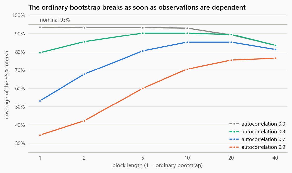
With independent data the ordinary bootstrap covers 94 percent, as advertised. At an autocorrelation of 0.3, which is mild, it covers 80 percent. At 0.7 it covers 53 percent: the nominal 95 percent interval misses the truth almost half the time. At 0.9 it is 34 percent, and the interval is close to worthless.
1
2
3
4
5
r = np.random.default_rng(1)
x = ar1(n, 0.7, r)
naive_sd = np.std([x[r.integers(0, n, n)].mean() for _ in range(2000)])
true_sd = np.std([ar1(n, 0.7, np.random.default_rng(10000 + s)).mean() for s in range(2000)])
print(f"phi = 0.7: naive bootstrap sd of the mean {naive_sd:.3f}; true sd {true_sd:.3f}; ratio {true_sd/naive_sd:.1f}")
The mechanism is in that ratio. At an autocorrelation of 0.7 the ordinary bootstrap believes the mean has a standard error of 0.076. Across genuinely independent series of the same process it is 0.234, three times larger for this series. Averaged over series the ordinary bootstrap gives 0.098, so the typical shortfall is a factor of 2.4. Positive autocorrelation means neighbouring points repeat each other's information, so 200 dependent points carry the information of roughly 200 times $(1-\phi)/(1+\phi)$ independent ones: about 35 at 0.7, about 10 at 0.9. The ordinary bootstrap counts 200.
Blocks recover most of the loss. At 0.7, blocks of 10 to 20 bring coverage to 85 percent; at 0.9, blocks of 20 to 40 reach 76 percent. Neither reaches 95, and the shortfall is not a bug in the method. With ten independent observations' worth of information, no resampling scheme can produce a well-calibrated interval, because the information is not there. The block bootstrap also has a cost visible in the first row: at zero autocorrelation, blocks of 40 give only five blocks per resample, the bootstrap distribution becomes lumpy, and coverage falls to 84 percent. Blocks should be long enough to contain the dependence and short enough to leave many of them. The rule of Hall, Horowitz and Jing is a length growing like $n^{1/3}$, about six here, and the stationary bootstrap of Politis and Romano, which draws random block lengths, removes the sharp dependence on the choice. When the dependence structure is known, fitting a time-series model and resampling its residuals is often better still.
Clustered Data
The same failure appears without any time axis. Thirty sites, twenty observations each, with a site effect that makes observations within a site correlated at 0.3, and a treatment applied to half the sites. The statistic is the treated-minus-control difference in means, and the truth is zero.
1
2
3
4
5
6
7
8
9
10
11
12
13
14
15
16
17
18
19
20
21
22
23
24
25
def cluster_data(r, clusters=30, per=20, icc=0.3, effect=0.0):
    site = np.repeat(np.arange(clusters), per)
    treated_site = np.arange(clusters) < clusters // 2
    u = r.normal(0, np.sqrt(icc), clusters)
    y = effect * treated_site[site] + u[site] + r.normal(0, np.sqrt(1 - icc), clusters * per)
    return y, site, treated_site[site].astype(float)

def diff(y, t):
    return y[t == 1].mean() - y[t == 0].mean()

cov_naive = cov_cluster = 0
reps = 500
for s in range(reps):
    r = np.random.default_rng(s)
    y, site, t = cluster_data(r)
    N = len(y)
    naive = [diff(*(lambda i: (y[i], t[i]))(r.integers(0, N, N))) for _ in range(400)]
    cl = []
    for _ in range(400):
        pick = r.integers(0, 30, 30)                                 # resample sites, not rows
        idx = np.concatenate([np.where(site == c)[0] for c in pick])
        cl.append(diff(y[idx], t[idx]))
    lo, hi = np.percentile(naive, [2.5, 97.5]); cov_naive += lo <= 0 <= hi
    lo, hi = np.percentile(cl, [2.5, 97.5]); cov_cluster += lo <= 0 <= hi
print(f"naive bootstrap 95% CI covers the truth in {cov_naive/reps:.0%} of datasets; cluster bootstrap {cov_cluster/reps:.0%}")
The ordinary bootstrap, resampling the 600 rows, covers the truth in 51 percent of datasets. Resampling the 30 sites instead, keeping each site's rows together, covers 90 percent.
The arithmetic is the design effect. With twenty observations per site and an intraclass correlation of 0.3, each site's rows are worth about $1 + 19 \times 0.3 = 6.7$ times less than independent rows, so the naive standard error is too small by a factor of $\sqrt{6.7}$, about 2.6. The treatment was assigned to sites, so sites are the independent units, and there are fifteen per arm. That is what the interval has to reflect, and the cluster bootstrap's remaining shortfall, 90 rather than 95, is the small-sample effect of having thirty clusters. With fewer than that, Cameron, Gelbach and Miller's wild cluster bootstrap is the standard remedy.
The general rule covers both cases so far: resample at the level at which the observations are independent. Rows within a site, days within a series, repeated measurements within a patient, and transactions within a customer are not independent of each other, and a bootstrap that resamples them one at a time will be confident and wrong.
Small Skewed Samples
The ordinary bootstrap can also fail with independent data, when the sample is small and the statistic's distribution is skewed. The percentile interval, which reads the 2.5th and 97.5th percentiles of the bootstrap distribution, is only accurate to first order, and with fifteen observations from a heavy-tailed distribution the second-order terms are not small.
1
2
3
4
5
6
7
8
9
10
11
12
13
14
15
16
17
reps, n = 2000, 15
true_mean = np.exp(0.5)                     # mean of a lognormal(0, 1)
cov_p = cov_t = 0
for s in range(reps):
    r = np.random.default_rng(s)
    x = r.lognormal(0, 1, n)
    m, se = x.mean(), x.std(ddof=1) / np.sqrt(n)
    bm, bt = [], []
    for _ in range(600):
        xb = x[r.integers(0, n, n)]
        bm.append(xb.mean())
        bt.append((xb.mean() - m) / (xb.std(ddof=1) / np.sqrt(n) + 1e-12))   # studentised
    lo, hi = np.percentile(bm, [2.5, 97.5])
    cov_p += lo <= true_mean <= hi
    q_lo, q_hi = np.percentile(bt, [2.5, 97.5])
    cov_t += (m - q_hi * se) <= true_mean <= (m - q_lo * se)
print(f"lognormal mean, n = 15: percentile interval covers {cov_p/reps:.0%}, bootstrap-t covers {cov_t/reps:.0%}")
The percentile interval covers 84 percent. The bootstrap-t interval, which bootstraps the studentised statistic and uses its quantiles to scale the standard error, covers 91 percent. The studentised version is second-order accurate: it adapts to the skewness of the sampling distribution instead of assuming it away, at the price of needing a standard error inside each resample. The bias-corrected and accelerated interval reaches the same order of accuracy without one and is the usual default in practice. Neither reaches 95 percent at fifteen observations from a distribution this skewed, and neither can: the sample simply does not contain the tail that determines the mean's variability.
Statistics at the Edge
There is a class of statistics for which the bootstrap fails outright, and the sample maximum is its cleanest member. Every bootstrap sample is drawn from the observed values, so no bootstrap maximum can exceed the observed maximum. The bootstrap distribution of the maximum is squashed against the observed value, and an interval read from it cannot reach the quantity the maximum estimates, which lies above it more often than not.
1
2
3
4
5
6
7
8
9
10
reps, n = 2000, 50
cov = 0
for s in range(reps):
    r = np.random.default_rng(s)
    x = r.exponential(1.0, n)
    bmax = [x[r.integers(0, n, n)].max() for _ in range(400)]
    lo, hi = np.percentile(bmax, [2.5, 97.5])
    true_q = -np.log(1 - 0.98)               # the 98th percentile, roughly what a max of 50 estimates
    cov += lo <= true_q <= hi
print(f"sample maximum of 50 exponentials: bootstrap 95% interval covers the 98th percentile in {cov/reps:.0%} of samples")
Coverage is 62 percent, and increasing the number of bootstrap replications does nothing, because the defect is in what the resamples can contain. Bickel and Freedman established the failure formally: the bootstrap is inconsistent for extreme order statistics. The same problem afflicts high quantiles, the range, and any statistic that depends on the edge of the sample. Those quantities need a model for the tail, which is the subject of extreme value theory, or a subsampling scheme that draws fewer than $n$ observations without replacement and rescales.
A milder version affects non-smooth statistics such as the median in small samples, whose bootstrap distribution takes only a handful of distinct values. It works asymptotically and is lumpy at small $n$; smoothing the bootstrap, or using a larger sample, is the fix.
Deciding Whether to Believe the Interval
- Ask how the data were generated before resampling anything. Time order, sites, subjects, customers and repeated measures are all forms of dependence, and the resampling unit has to be the independent one.
- For series, use blocks of length near $n^{1/3}$, or the stationary bootstrap, and expect coverage to fall short when the series is short relative to its dependence.
- For clusters, resample clusters, and switch to the wild cluster bootstrap when there are fewer than about thirty.
- For small or skewed samples, use bootstrap-t or the bias-corrected and accelerated interval rather than the percentile interval, by default rather than by exception.
- Do not bootstrap maxima, minima, ranges or extreme quantiles. Fit a tail model instead.
- Check by simulation. Generate data from a process that resembles yours, with the dependence you suspect, and measure the coverage of the interval you plan to report. An hour of computation replaces an assumption that cannot otherwise be checked, and it is how every number in this post was obtained.
The bootstrap is not assumption-free. It has one assumption, and it is the one about how the data arose, which is also the one most often untrue.
The figure generator in the blog-reproducibility repository reproduces this article's figure; run it with --dry-run to print the numbers behind the figure without writing an image.
References
- Efron, B. (1979). Bootstrap methods: another look at the jackknife. The Annals of Statistics, 7(1), 1-26.
- Efron, B., & Tibshirani, R. J. (1993). An Introduction to the Bootstrap. Chapman and Hall.
- Davison, A. C., & Hinkley, D. V. (1997). Bootstrap Methods and Their Application. Cambridge University Press.
- Künsch, H. R. (1989). The jackknife and the bootstrap for general stationary observations. The Annals of Statistics, 17(3), 1217-1241.
- Politis, D. N., & Romano, J. P. (1994). The stationary bootstrap. Journal of the American Statistical Association, 89(428), 1303-1313.
- Hall, P., Horowitz, J. L., & Jing, B.-Y. (1995). On blocking rules for the bootstrap with dependent data. Biometrika, 82(3), 561-574.
- Cameron, A. C., Gelbach, J. B., & Miller, D. L. (2008). Bootstrap-based improvements for inference with clustered errors. The Review of Economics and Statistics, 90(3), 414-427.
- Bickel, P. J., & Freedman, D. A. (1981). Some asymptotic theory for the bootstrap. The Annals of Statistics, 9(6), 1196-1217.
Embed interactive plots, widgets, and demos using <figure>, <iframe>, or <div class="interactive-embed"> containers. Ensure each embed includes descriptive captions for accessibility.
How to cite
Use the quick export buttons to save citations for reference managers or copy the formatted text directly.
Diogo Ribeiro (2026). When the Bootstrap Fails: Dependent Data, Small Samples, and Extremes. Faculty of Media Arts and Design, Technical University of Porto. https://diogoribeiro7.github.io/statistics/bootstrap_dependent_data_when_it_fails/.

