Topics
The satisfaction survey came back at 7.36 out of ten, up from last quarter, and went into the board pack. The true population figure is 7.10. Every response was honest and the arithmetic was right.
What went wrong is who answered. Older customers responded at twice the rate of younger ones, and older customers are more satisfied. The sample is a fair picture of the people who reply to surveys and a distorted picture of the customer base. The distortion is fixable, because the age distribution of the customer base is already known.
A Population and an Uneven Response
1
2
3
4
5
6
7
8
9
10
11
12
13
14
15
16
17
18
19
20
21
22
23
24
25
26
27
28
29
30
31
32
33
34
35
36
37
38
39
40
41
42
43
44
45
46
47
48
49
50
51
52
53
54
55
56
57
58
59
60
61
62
63
64
65
66
67
68
69
70
71
72
73
74
75
76
77
import numpy as np

RNG = np.random.default_rng(73)
POP = 200_000
AGES = np.array([0.28, 0.27, 0.25, 0.20])          # population shares, four age bands
REGIONS = np.array([0.50, 0.30, 0.20])
SCORE = np.array([[6.0, 6.4, 6.8],                  # mean score by age and region
                  [6.6, 7.0, 7.4],
                  [7.2, 7.6, 8.0],
                  [7.8, 8.2, 8.6]])


def population(n=POP, rng=RNG):
    age = rng.choice(4, n, p=AGES)
    region = rng.choice(3, n, p=REGIONS)
    keen = rng.normal(0, 1, n)                      # an attitude nobody measures
    y = SCORE[age, region] + 0.7 * keen + rng.normal(0, 1.0, n)
    return age, region, keen, y


def respond(age, keen, by_attitude=0.0, rng=RNG):
    """Older people answer more often; optionally the keen answer more too."""
    logit = -1.6 + 0.55 * age + by_attitude * keen
    return rng.random(age.size) < 1 / (1 + np.exp(-logit))


def post_stratify(age, region, y, joint=False):
    """Reweight each cell to its known share of the population."""
    if joint:
        cells = age * 3 + region
        target = np.outer(AGES, REGIONS).ravel()
    else:
        cells = age
        target = AGES
    w = np.zeros(y.size)
    for c, share in enumerate(target):
        m = cells == c
        if m.sum():
            w[m] = share / (m.sum() / y.size)
    return np.average(y, weights=w), w


def rake(age, region, y, rounds=12):
    """Only the margins are known, so scale to one, then the other, repeatedly."""
    w = np.ones(y.size)
    for _ in range(rounds):
        for var, target in ((age, AGES), (region, REGIONS)):
            for c, share in enumerate(target):
                m = var == c
                if m.sum():
                    w[m] *= share / (w[m].sum() / w.sum())
    return np.average(y, weights=w), w


def kish(w):
    """Effective sample size after weighting."""
    return w.sum() ** 2 / np.sum(w ** 2)


age, region, keen, y = population()
TRUE = y.mean()
r = np.random.default_rng(5)
sel = respond(age, keen, rng=r)
print(f"population mean {TRUE:.4f}")
print(f"responded: {sel.sum():,} people, {sel.mean():.1%} of the population")
print("age shares among respondents " + ", ".join(
    f"{np.mean(age[sel] == a):.0%}" for a in range(4)))
naive = y[sel].mean()
ps_age, w_age = post_stratify(age[sel], region[sel], y[sel])
ps_joint, w_joint = post_stratify(age[sel], region[sel], y[sel], joint=True)
rk, w_rk = rake(age[sel], region[sel], y[sel])
for name, val, w in (("unweighted", naive, np.ones(sel.sum())),
                     ("weighted on age", ps_age, w_age),
                     ("weighted on age and region jointly", ps_joint, w_joint),
                     ("raked to both margins", rk, w_rk)):
    print(f"{name:36s} {val:.4f}  bias {val - TRUE:+.4f}  "
          f"effective sample {kish(w):8,.0f} of {sel.sum():,}")
The population splits 28, 27, 25 and 20 percent across four age bands and has a mean score of 7.097. Among the 62,706 people who answered, the age shares are 15, 22, 30 and 33 percent: the oldest band is over-represented by two thirds.
| Estimate | Value | Bias | Effective sample |
|---|---|---|---|
| Unweighted | 7.3609 | +0.2639 | 62,706 |
| Weighted on age | 7.1006 | +0.0036 | 53,248 |
| Weighted on age and region jointly | 7.1011 | +0.0041 | 53,245 |
| Raked to both margins | 7.1011 | +0.0042 | 53,248 |
Weighting removes the bias almost entirely. The mechanism is simple enough to write out: each respondent counts as the number of people in the population their cell represents, divided by the number of respondents in that cell, so an under-represented band gets a weight above one and an over-represented band below one.
The three weighted estimates agree because age and region are independent here. When they are not, weighting on age alone leaves the region imbalance untouched, and the joint version fixes both at the cost of needing the full cross-classification of the population.
Raking, When Only the Margins Are Known
The joint distribution is often unavailable. A company knows its age distribution and its regional distribution but not how many customers are both young and in the third region. Raking solves this by scaling to one margin, then the other, and repeating until both hold.
In the table above raking matches the joint result to four decimal places. That agreement is a property of this population, where the two variables are independent; when they are correlated, raking reproduces the margins but not the interior of the table, and the remaining bias depends on how much the outcome varies within cells that raking cannot distinguish.
What the Weights Cost
Weighting is not free. Unequal weights make the estimate noisier, and the standard measure of how much is Kish's effective sample size, which is the number of equally weighted observations that would give the same precision.
1
2
3
4
5
6
7
8
9
for slope in (0.2, 0.55, 1.0, 1.5):
    r = np.random.default_rng(11)
    logit = -1.6 + slope * age
    s = r.random(age.size) < 1 / (1 + np.exp(-logit))
    v, w = post_stratify(age[s], region[s], y[s])
    ratio = w.max() / w.min()
    print(f"response slope {slope:4.2f}: youngest respond {np.mean(s[age == 0]):5.1%}, "
          f"oldest {np.mean(s[age == 3]):5.1%}, weight ratio {ratio:5.2f}, "
          f"effective sample {kish(w) / s.sum():5.0%} of respondents, bias {v - TRUE:+.4f}")
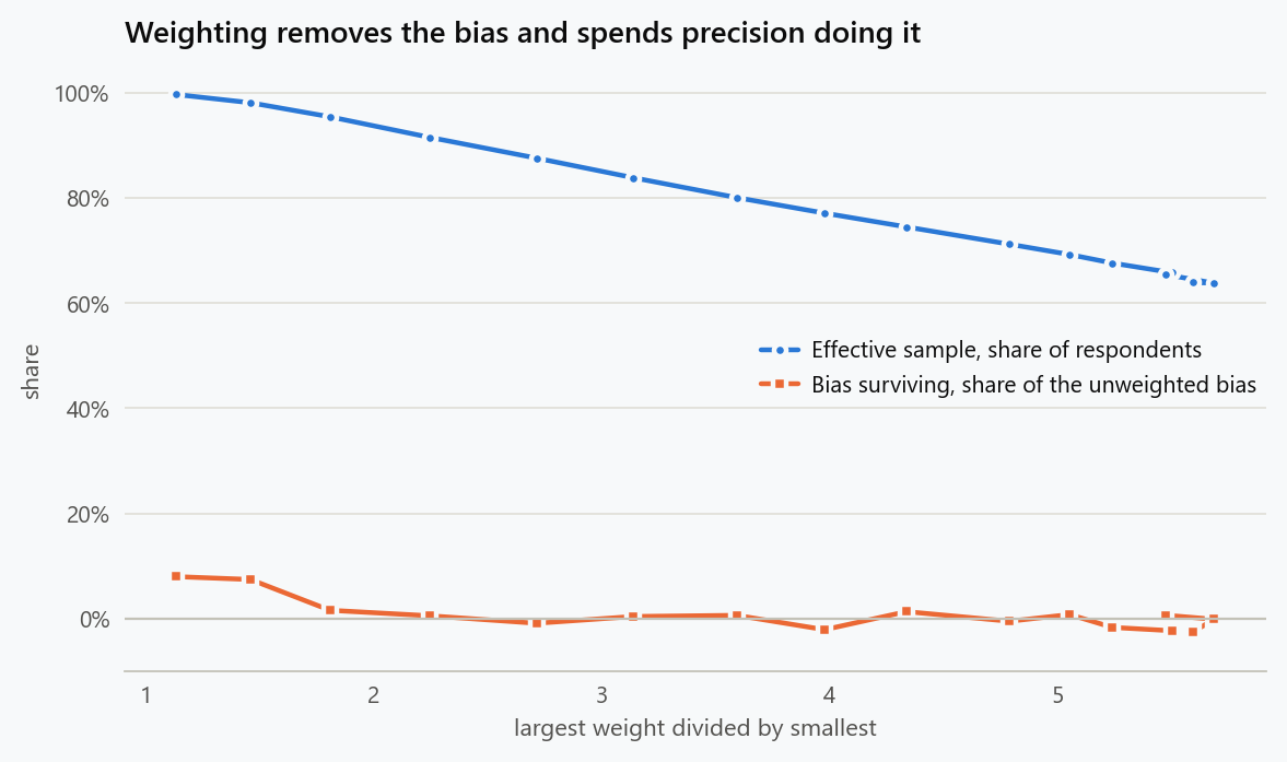
| Imbalance | Youngest respond | Oldest respond | Largest weight over smallest | Effective sample | Bias after weighting |
|---|---|---|---|---|---|
| Mild | 16.6% | 26.5% | 1.59 | 97% | +0.0034 |
| Moderate | 16.6% | 50.8% | 3.04 | 85% | +0.0063 |
| Severe | 16.6% | 79.8% | 4.77 | 71% | +0.0045 |
| Extreme | 16.6% | 94.6% | 5.65 | 64% | +0.0010 |
The bias is removed at every level of imbalance, and the price is precision. At the moderate imbalance that matches the survey above, weighting keeps 85 percent of the sample as effective observations, so a survey of 1,000 answers behaves like 850. At the extreme, a third of the sample's value is gone.
That is the right trade in almost every case, because bias does not shrink with sample size and variance does. But it has a planning consequence: a survey that will need heavy weighting should be sized for its effective sample, not its response count.
The Limit That Matters
Weighting corrects imbalance in the variables used to build the weights. If response depends on something else, the correction addresses only the part of that dependence which happens to run through the weighting variables.
1
2
3
4
5
6
7
8
9
10
11
12
13
14
15
16
17
18
19
20
21
for by_attitude in (0.0, 0.5):
    rows = {k: [] for k in ("unweighted", "age", "joint", "raked")}
    eff = []
    for i in range(300):
        r = np.random.default_rng(1000 + i)
        s = respond(age, keen, by_attitude=by_attitude, rng=r)
        rows["unweighted"].append(y[s].mean() - TRUE)
        rows["age"].append(post_stratify(age[s], region[s], y[s])[0] - TRUE)
        v, w = post_stratify(age[s], region[s], y[s], joint=True)
        rows["joint"].append(v - TRUE)
        v2, w2 = rake(age[s], region[s], y[s])
        rows["raked"].append(v2 - TRUE)
        eff.append(kish(w2) / s.sum())
    label = "response depends on age only" if by_attitude == 0 else \
            "response also depends on the unmeasured attitude"
    print(f"{label}:")
    for k, v in rows.items():
        v = np.array(v)
        print(f"  {k:12s} bias {v.mean():+.4f}, spread {v.std():.4f}, "
              f"root mean squared error {np.sqrt(np.mean(v ** 2)):.4f}")
    print(f"  weighting keeps {np.mean(eff):.0%} of the sample as effective observations")
| Estimate | Bias when response depends on age only | Bias when it also depends on an unmeasured attitude |
|---|---|---|
| Unweighted | +0.2604 | +0.4582 |
| Weighted on age | +0.0005 | +0.2291 |
| Weighted jointly | +0.0014 | +0.2297 |
| Raked | +0.0014 | +0.2297 |
In the first column weighting is essentially exact. In the second, where enthusiasm about the product also drives whether people answer, weighting removes half the bias and leaves the other half in place, because no amount of reweighting on age can distinguish a satisfied customer who answered from a satisfied customer who did not.
This is the honest limit of the method, and it is why a weighted survey is not the same as a representative one. The weights make the sample match the population on the things used to build them. Everything else is an assumption, and the assumption is that within an age band and region, the people who answered are like the people who did not.
Reducing the Part Weighting Cannot Reach
Since the residual bias comes from unmeasured response behaviour, the leverage is in the response process rather than in the arithmetic afterwards. Raising the overall response rate shrinks the gap between respondents and non-respondents mechanically, because there is less room for them to differ. Chasing a random subsample of non-respondents gives a direct measurement of that difference. And collecting a variable that predicts both the answer and the response, such as tenure or recent usage, brings part of the hidden mechanism into the weighting scheme.
None of those is free, and all three are more useful than adding a fourth weighting variable that everybody already responds on evenly.
What to Do
- Compare the sample's composition against the population on every variable you have, before looking at the outcome. That comparison is the diagnostic, and it takes one query.
- Weight to the joint distribution when you have it, and rake to the margins when you do not.
- Report the effective sample size next to the weighted estimate, and use it for every interval and test.
- Size surveys for the effective sample. Heavy weighting can cost a third of the responses.
- Do not describe a weighted survey as representative. Say what it was weighted on, because that is exactly the extent of the claim.
- Spend effort on response rates and on non-respondent follow-up rather than on more weighting variables, because that is the only way to reach the bias that weighting cannot.
The figure generator in the blog-reproducibility repository reproduces this article's figure; run it with --dry-run to print the numbers behind the figure without writing an image.
References
- Holt, D., & Smith, T. M. F. (1979). Post stratification. Journal of the Royal Statistical Society: Series A, 142(1), 33-46.
- Kish, L. (1965). Survey Sampling. Wiley.
- Deming, W. E., & Stephan, F. F. (1940). On a least squares adjustment of a sampled frequency table when the expected marginal totals are known. Annals of Mathematical Statistics, 11(4), 427-444.
- Little, R. J. A. (1993). Post-stratification: a modeler's perspective. Journal of the American Statistical Association, 88(423), 1001-1012.
- Gelman, A. (2007). Struggles with survey weighting and regression modeling. Statistical Science, 22(2), 153-164.
- Groves, R. M., & Peytcheva, E. (2008). The impact of nonresponse rates on nonresponse bias: a meta-analysis. Public Opinion Quarterly, 72(2), 167-189.
Embed interactive plots, widgets, and demos using <figure>, <iframe>, or <div class="interactive-embed"> containers. Ensure each embed includes descriptive captions for accessibility.
How to cite
Use the quick export buttons to save citations for reference managers or copy the formatted text directly.
Diogo Ribeiro (2026). Post-Stratification: Weighting a Survey That Answered Unevenly. Faculty of Media Arts and Design, Technical University of Porto. https://diogoribeiro7.github.io/statistics/post_stratification_weighting_a_survey/.

