DPO Changes Preferences, Not Knowledge

Supervised fine-tuning and preference optimization are often described as consecutive stages of the same recipe:

Operationally, that sequence is common. Statistically, the stages learn from different objects.

Supervised fine-tuning observes a target response

and increases the probability of that response.

Preference optimization observes a comparison

where $y^+$ is preferred to $y^-$ under some annotation process.

The distinction matters because a preference label does not say that $y^+$ is objectively correct. It says that, given the prompt and the alternatives presented, one response was preferred.

That preference may reflect factual accuracy, helpfulness, tone, brevity, safety, style, formatting, social norms, annotator expectations, or some mixture of all of them.

DPO is therefore best understood as a method for changing relative response preferences.

It is not a knowledge-ingestion mechanism.

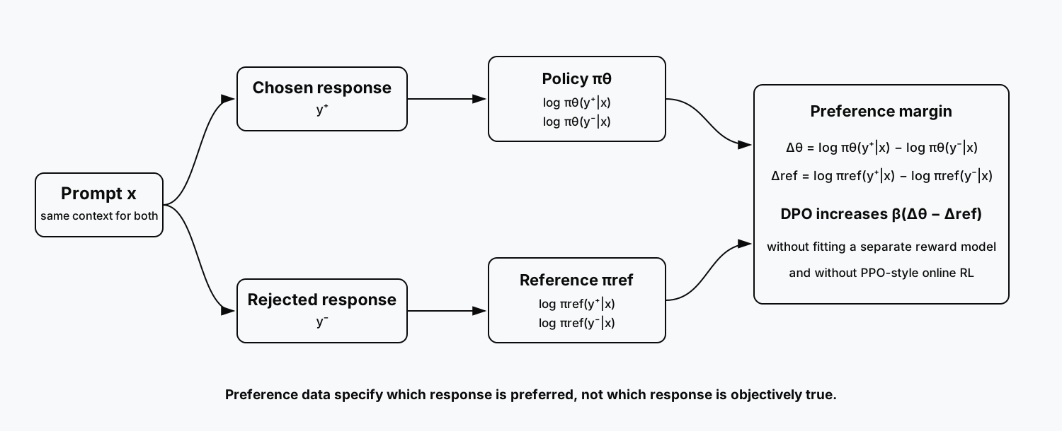
The key quantity is not the raw probability of the chosen response. It is the chosen-versus-rejected log-odds under the policy relative to the same margin under a reference model.

Preference data are pairwise observations

Let a prompt be

with two candidate responses

and

The observed label is

meaning that the chosen response was preferred to the rejected response.

A preference dataset is therefore

This is not equivalent to an SFT dataset containing only

The rejected response carries information about the decision boundary.

Consider two pairs:

1. a perfect answer versus a completely irrelevant answer,
2. a strong answer versus a slightly stronger answer.

Both have one chosen and one rejected response.

The second pair is much harder.

A binary preference label alone does not encode that difficulty unless the model can infer it from the response probabilities and content.

This is one reason preference-data quality matters so much.

The Bradley-Terry model gives the basic preference likelihood

A common pairwise preference model assumes an unobserved reward function

Under a Bradley-Terry-style model,

where

The probability of preferring one response depends on the difference between their latent rewards.

Traditional RLHF often fits a reward model from these pairwise labels and then optimizes the policy against that learned reward using reinforcement learning while constraining the policy from drifting too far from a reference model.

DPO avoids fitting a separate reward model explicitly.

DPO rewrites the reward in terms of policy ratios

The regularized RLHF objective can be written schematically as

The KL term penalizes movement away from a reference policy

For the corresponding optimal policy,

Rearranging gives the reward up to a prompt-dependent normalizing constant:

For a pairwise difference, the normalization term cancels:

This is the central DPO transformation.

Instead of fitting a reward model and then running PPO or another reinforcement-learning algorithm, DPO directly optimizes the policy so that preferred responses receive a larger relative margin than rejected responses.

The DPO loss is a logistic preference loss

Define the policy preference margin

and the reference margin

The DPO logit is

The standard loss is

Training therefore pushes

for chosen-versus-rejected pairs.

The policy is not merely being told that the chosen response is probable.

It is being told to increase its relative preference for the chosen response compared with the reference policy.

The reference model anchors the update

The reference policy is not an incidental implementation detail.

Suppose the chosen response already has much higher probability than the rejected response under the reference model.

Then

is already large.

The policy must improve relative to that existing margin.

Conversely, if the reference strongly prefers the rejected response, the policy must overcome that baseline.

This anchoring prevents DPO from being equivalent to ordinary pairwise classification over the policy alone.

In practice, the reference model is often the model state before DPO begins, commonly an SFT checkpoint.

Current TRL can use the initial policy state automatically when no explicit reference model is supplied. citeturn345825search0

Beta controls the strength of the reference constraint

The hyperparameter

appears directly in the preference logit.

It is often described as a KL-control parameter.

Intuitively:

• smaller effective regularization allows more aggressive movement,
• stronger reference regularization keeps the policy closer to the reference behaviour.

The exact interpretation depends on the formulation and implementation, but the important practical point is that beta changes the trade-off between preference fitting and policy drift.

It should not be copied blindly.

A useful sweep might compare

The evaluation should track not only preference accuracy but also regressions on unrelated capabilities.

A model can fit preference pairs better while becoming worse in deployment.

DPO should usually start from a competent SFT model

Preference optimization is not a substitute for basic instruction following.

Suppose the base model cannot reliably:

• follow the chat protocol,
• produce coherent responses,
• emit the required output structure,
• understand the domain vocabulary.

Pairwise preference training is an awkward way to teach those fundamentals.

SFT provides direct demonstrations.

DPO then changes relative preference among plausible responses.

This suggests a division of labour:

The boundary is not absolute, but it is conceptually useful.

A chosen response is not automatically a good response

Preference datasets often invite a dangerous simplification:

chosen = correct, rejected = wrong.

That need not be true.

Imagine the pair:

Chosen: a concise answer with one subtle factual error.

Rejected: a correct answer that is verbose and awkward.

An annotator instructed to prefer concise answers may choose the first.

DPO will then learn exactly what the data say.

The algorithm cannot recover an objective the annotation process did not encode.

This is why preference optimization is fundamentally a measurement problem.

Let the true deployment utility be

while the annotation process produces preferences according to

If

is only weakly aligned with

then optimizing annotation preferences can reduce deployment utility.

Preference criteria should be explicit

Before collecting data, define what preference means.

Possible dimensions include:

• factual correctness,
• completeness,
• concision,
• style,
• citation quality,
• policy compliance,
• harmlessness,
• tool-use correctness,
• uncertainty calibration.

If several dimensions are mixed into one binary label, disagreements become hard to interpret.

A useful annotation record may include both a pairwise decision and dimension-level judgments.

For example:

1
2
3
4
5
6
7
8
{
  "prompt_id": "p-1042",
  "chosen": "A",
  "factuality": "A",
  "completeness": "tie",
  "style": "B",
  "policy_compliance": "A"
}

The overall chosen label may still be used for DPO, but the extra fields reveal why the preference occurred.

They also support stratified evaluation later.

Inter-annotator disagreement is information

If two qualified annotators disagree frequently, the problem may be genuinely ambiguous.

For pair $i$, let

Pairs with

are intrinsically uncertain under the annotation population.

Collapsing repeated judgments into a deterministic label discards that uncertainty.

Possible responses include:

• collect more labels,
• remove ambiguous pairs,
• preserve soft preference probabilities,
• model annotator heterogeneity,
• evaluate sensitivity to label noise.

DPO does not make disagreement disappear.

It converts the observed labels into gradient updates.

Position bias can contaminate pairwise labels

If candidate A is always displayed first and candidate B second, annotators may exhibit order effects.

The observed preference then depends on both content and presentation.

A basic annotation design should randomize left-right or first-second order.

If

position bias exists.

That bias becomes training signal if not controlled.

Randomization is cheap here. There is little excuse not to use it.

Length bias deserves explicit testing

Preference datasets often favour longer answers because longer responses appear more thorough.

Or they favour shorter answers because annotators are instructed to prefer concision.

Either way, response length can become a shortcut.

Let

Inspect the distribution of

If chosen responses are systematically longer, DPO can increase verbosity even when verbosity is not the target.

Evaluate preference performance conditionally on length difference.

A simple diagnostic is a logistic model:

A large length coefficient is not proof of bias, but it is a signal worth investigating.

Pair difficulty matters

If the chosen and rejected responses are nearly identical, the label is subtle.

If one is excellent and the other nonsense, the label is trivial.

A preference dataset containing mostly trivial negatives can yield high training accuracy while teaching little about difficult distinctions.

Hard negative construction therefore matters.

Useful rejected responses may come from:

• weaker model checkpoints,
• alternative decoding temperatures,
• prompt perturbations,
• known failure modes,
• human-written near misses.

The rejected response should be plausible enough that the comparison teaches the intended preference boundary.

Train, validation and test splits must preserve pair dependencies

Preference data often come from a shared prompt pool.

A single prompt may have several candidate responses and several pairwise comparisons.

All comparisons from the same prompt should usually remain in the same split.

Let

A leakage-safe split requires

If one response pair from a prompt is in training and another nearly identical pair is in test, the test set is not independent in the useful sense.

The same principle applies when prompts are generated from common documents or templates.

A current conversational DPO dataset is simple

Current TRL supports explicit conversational prompts with chosen and rejected assistant responses. citeturn345825search0

A record can look like:

1
2
3
4
5
6
7
8
9
10
11
12
13
14
15
16
17
18
19
20
example = {
    "prompt": [
        {
            "role": "user",
            "content": "Explain why a confidence interval is not a probability statement about a fixed parameter."
        }
    ],
    "chosen": [
        {
            "role": "assistant",
            "content": "In frequentist inference, the parameter is treated as fixed..."
        }
    ],
    "rejected": [
        {
            "role": "assistant",
            "content": "There is a 95% probability that the true parameter lies inside..."
        }
    ],
}

The chosen and rejected responses share the same prompt.

The trainer applies the chat template for conversational data.

As with SFT, inspect the rendered tokens before training.

DPO can be combined with LoRA or QLoRA

Preference optimization changes the objective.

LoRA changes the parameterization of the update.

They are independent design dimensions.

A parameter-efficient DPO configuration can therefore use PEFT:

1
2
3
4
5
6
7
8
9
10
11
12
13
14
15
16
17
18
19
20
21
22
23
24
25
26
27
28
29
30
31
32
33
34
35
36
37
38
39
40
41
42
43
44
45
46
47
48
49
50
51
52
53
54
55
56
57
from datasets import load_dataset
from peft import LoraConfig
from trl import DPOConfig, DPOTrainer


model_id = "your-sft-model"

dataset = load_dataset(
    "json",
    data_files={
        "train": "preferences_train.jsonl",
        "validation": "preferences_validation.jsonl",
    },
)


peft_config = LoraConfig(
    r=16,
    lora_alpha=32,
    lora_dropout=0.05,
    target_modules="all-linear",
    bias="none",
    task_type="CAUSAL_LM",
)


args = DPOConfig(
    output_dir="outputs/dpo-adapter",
    num_train_epochs=1,
    per_device_train_batch_size=2,
    per_device_eval_batch_size=2,
    gradient_accumulation_steps=8,
    learning_rate=5e-6,
    beta=0.1,
    max_length=2048,
    eval_strategy="steps",
    eval_steps=100,
    save_strategy="steps",
    save_steps=100,
    logging_steps=10,
    bf16=True,
    gradient_checkpointing=True,
    report_to="none",
)


trainer = DPOTrainer(
    model=model_id,
    args=args,
    train_dataset=dataset["train"],
    eval_dataset=dataset["validation"],
    peft_config=peft_config,
)


trainer.train()
trainer.save_model("outputs/dpo-adapter/final")

The numerical values are starting points, not recommendations.

The current TRL interface supports PEFT wrapping directly and can use the initial policy as the reference when ref_model is not supplied. citeturn345825search0

QLoRA is also possible for DPO

If memory is limiting, the policy can be loaded quantized while training LoRA adapters.

Current DPOTrainer accepts both a quantization configuration and a PEFT configuration when the model is provided by identifier. citeturn345825search0

For example:

1
2
3
4
5
6
7
8
9
10
11
12
13
14
15
16
17
18
19
20
21
import torch

from transformers import BitsAndBytesConfig


quantization_config = BitsAndBytesConfig(
    load_in_4bit=True,
    bnb_4bit_quant_type="nf4",
    bnb_4bit_use_double_quant=True,
    bnb_4bit_compute_dtype=torch.bfloat16,
)


trainer = DPOTrainer(
    model=model_id,
    args=args,
    train_dataset=dataset["train"],
    eval_dataset=dataset["validation"],
    peft_config=peft_config,
    quantization_config=quantization_config,
)

This changes memory usage.

It does not change the DPO objective.

Precomputing reference log-probabilities can save memory

DPO needs both policy and reference log-probabilities.

If the reference model is fixed, its log-probabilities can be computed ahead of time rather than recomputed every step.

Current TRL exposes

1
precompute_ref_log_probs=True

for this purpose. citeturn908884search0

This can reduce memory pressure because the reference model does not need to remain resident during every training step.

The trade-off is preprocessing time and storage of reference scores.

Again, this is an engineering optimization, not a change to the estimand.

Preference accuracy is not enough

A DPO trainer can report whether the policy assigns a larger reward margin to chosen than rejected responses.

High pairwise preference accuracy on the validation set is useful.

It does not establish that free-form generations improved.

The model can overfit pairwise distinctions without producing better responses when sampled independently.

Evaluation should therefore include at least two layers:

1. pairwise held-out preference performance,
2. generated-response evaluation on independent prompts.

The second layer is the deployment-relevant one.

Evaluate against the SFT checkpoint

The most important baseline is often the model immediately before DPO.

Compare:

Use the same generation parameters.

Evaluate:

• target preference dimensions,
• factuality,
• task accuracy,
• style,
• verbosity,
• safety or refusal behaviour,
• unrelated regression tasks.

If DPO increases the chosen-response win rate but damages factual accuracy, the preference dataset may be rewarding the wrong thing.

Blind pairwise evaluation is natural for DPO

For open-ended behaviour, human pairwise evaluation is often easier than absolute scoring.

Generate one answer from each model:

Randomize presentation order and ask evaluators to choose:

• A,
• B,
• tie,
• both unacceptable.

The estimated win probability is

Report uncertainty.

A 52% win rate on 50 prompts is not compelling evidence of improvement.

DPO can amplify annotator style preferences

Suppose annotators consistently favour:

• headings,
• bullet lists,
• assertive tone,
• long explanations.

DPO can learn those surface preferences extremely well.

The resulting model may appear more polished while factual performance remains unchanged.

This is especially dangerous when using an LLM-as-judge to generate preference labels because the judge may favour its own stylistic conventions.

Preference optimization can therefore create a feedback loop:

That loop can improve benchmark scores without improving user utility.

LLM-generated preference data should be treated as noisy measurements

RLAIF replaces or supplements human preferences with AI-generated feedback.

This can scale data collection dramatically.

It also transfers the evaluator model's biases into the training set.

If an LLM judge produces label

for latent desired preference

then

is a measurement-error rate.

That error may depend on topic, length, style and model identity.

It is not generally random.

A serious RLAIF pipeline should validate a stratified sample against qualified human judgment.

Reference choice changes the problem

The reference model determines what counts as policy drift.

Using the original pretrained base versus the SFT checkpoint creates different anchors.

If DPO follows SFT, the natural reference is often the SFT model.

Then DPO asks:

How should the SFT policy change to better match the preference data?

Using a much earlier reference changes that comparison.

The reference model should therefore be documented explicitly.

DPO does not guarantee a fixed KL distance

Beta is connected to KL regularization in the derivation, but setting beta does not mean the final trained policy will achieve one predetermined KL divergence on every deployment prompt.

Measure actual drift.

Useful diagnostics include held-out estimates of

or simpler proxies such as log-probability shifts on evaluation sequences.

The practical question is whether the policy changed more broadly than intended.

Preference overfitting can happen before token-level overfitting looks dramatic

The DPO objective can memorize pairwise distinctions.

If the number of prompts is small, training accuracy may approach one rapidly.

The important question is whether the preference rule generalizes to new prompts and new candidate responses.

Split by prompt identity and maintain a final generation test set.

Do not use the training preference pairs as evidence that the deployed policy is aligned.

DPO cannot fix missing information

Suppose both chosen and rejected responses are based on incomplete knowledge.

Preference optimization can make the model prefer the less bad answer.

It cannot create a missing fact reliably.

If the actual problem is that the model lacks access to current information, use retrieval or another knowledge-access mechanism.

This returns to the broader taxonomy:

The methods address different failure mechanisms.

IPO changes the statistical assumptions

DPO is not the only direct preference objective.

Identity Preference Optimization and related work examine alternative losses and regularization structures.

The practical lesson is not that one objective universally dominates another.

It is that preference optimization embeds assumptions about how observed choices relate to latent utility and how strongly the policy should move.

The choice of loss belongs in the model specification.

It should not be hidden behind a trainer default.

KTO can learn from desirable and undesirable examples without explicit pairs

KTO takes a different route.

Instead of requiring a chosen and rejected response for the same prompt, it can use binary signals indicating whether an output is desirable or undesirable.

The method is motivated by a prospect-theoretic utility view and belongs to a broader family of human-aware losses. Its authors explicitly argue that no one such objective is universally best; the appropriate inductive bias depends on the setting. citeturn908884academia12

This can be operationally attractive when pair generation is expensive.

But binary desirability labels are still measurements of a preference process.

They do not escape the data-quality problem.

Preference optimization should be evaluated as causal intervention on behaviour

The deployment question is not

Did DPO loss decrease?

It is

Did applying DPO to the SFT checkpoint cause an improvement in the behaviours we care about without unacceptable regressions?

That is an experimental comparison.

Let

denote the score for prompt $i$ under the DPO policy and

the score under the SFT reference.

On a fixed paired evaluation set, define

Then estimate

For human pairwise evaluation, the equivalent object may be the win probability.

The important point is that preference training itself is not the outcome.

Behavioural change is the outcome.

Release criteria should be multidimensional

A DPO model should not be released merely because it wins one preference benchmark.

A release rule might require:

while also requiring

and

The exact thresholds depend on the application.

The structure matters more than the numbers.

Preference optimization changes a model along several dimensions simultaneously.

The hardest DPO problem is deciding whose preferences are being optimized

The notation

looks objective.

It is not.

Someone or something produced that comparison.

A human annotation workforce, domain experts, customers, an LLM judge, a policy document, or a mixture of sources defines what "preferred" means.

Different populations can have different utility functions.

Let

denote preferences for annotator population $a$ and

for population $b$.

There is no reason these must be equal.

A model optimized for one preference population may systematically frustrate another.

Preference optimization is therefore not merely an optimization problem.

It is also a target-population problem.

DPO is simpler than PPO-based RLHF, not assumption free

The original attraction of DPO is real.

It removes a large amount of machinery:

• no separately trained reward model in the basic pipeline,
• no PPO loop,
• no online sampling during optimization in the original formulation,
• no explicit reward-maximization stage.

That simplicity is valuable. The original paper demonstrated strong results while substantially simplifying the RLHF pipeline. citeturn908884academia13

But simplicity of optimization does not imply simplicity of measurement.

The preference labels still define the target.

The reference model still defines the anchor.

Beta still controls the update geometry.

Dataset construction still determines what behaviours are visible.

Evaluation still determines whether anything useful improved.

DPO removes infrastructure.

It does not remove experimental design.

References

Azar, M. G., Rowland, M., Piot, B., Guo, D., Calandriello, D., Valko, M., & Munos, R. (2024). A General Theoretical Paradigm to Understand Learning from Human Preferences. Proceedings of AISTATS 2024.

Ethayarajh, K., Xu, W., Muennighoff, N., Jurafsky, D., & Kiela, D. (2024). KTO: Model Alignment as Prospect Theoretic Optimization. Proceedings of ICML 2024.

Hugging Face. TRL documentation: DPO Trainer. Accessed 20 September 2026.

Rafailov, R., Sharma, A., Mitchell, E., Ermon, S., Manning, C. D., & Finn, C. (2023). Direct Preference Optimization: Your Language Model Is Secretly a Reward Model. Advances in Neural Information Processing Systems, 36.