Advanced Sequential Change-Point Detection for Univariate Models

Corrected on 19 September 2026: repaired equation formatting and the incomplete Python example, and reconciled the CUSUM definitions. The original archive date is retained.

Overview

A sequential detector must decide whether to raise an alarm using only the observations available now. It cannot inspect the rest of the series before deciding that an earlier observation looked unusual.

That makes its output different from an offline segmentation. A segmentation estimates where a series changed after observing a chosen window. A sequential procedure reports when accumulated evidence first crosses a decision threshold. The alarm usually arrives after the underlying change, and can also arrive before any change as a false alarm.

This article develops a consistent example: independent Gaussian measurements whose mean may increase by a specified amount. We derive the CUSUM update from a likelihood ratio, distinguish one-sided and two-sided monitoring, compare the structure with Shiryaev–Roberts, and run a complete Python example. The threshold is illustrative; a successful plot does not establish an acceptable false-alarm rate.

Theoretical Foundations

Change-Point Model

Let $X_1,X_2,\ldots$ arrive in order. Define $\tau$ as the index of the last observation before the change, so the first changed observation is $X_{\tau+1}$:

For the derivation, observations are independent conditional on the change location, and the pre-change and post-change densities $f_0$ and $f_1$ are specified. The no-change case is denoted by $\tau=\infty$.

These assumptions have operational meaning. A seasonal series cannot usually be treated as independent draws around one fixed mean. If the baseline is fitted from data, its estimation uncertainty also becomes part of the monitoring problem. Here we hold the baseline and variance fixed to make the detector's mechanism inspectable.

Hypothesis Testing Framework

At time $n$, compare no change through time $n$ with a change after a candidate observation $k$, where $0\le k<n$. The value $k=0$ allows a change before the first observation in the monitoring window.

For that candidate location, the likelihood ratio is

Define the log-likelihood increment $\ell_t=\log[f_1(X_t)/f_0(X_t)]$. Then $\log L_{k,n}=\sum_{t=k+1}^{n}\ell_t$. This is a likelihood ratio, not a posterior probability that a change has occurred.

Maximising over possible locations handles the unknown $k$. If the post-change distribution also contains unknown parameters, maximising over those parameters creates a different, more complex procedure. The fixed-density recursion below should not be silently reused as though it solved every such problem.

Advanced Methods for Sequential Change-Point Detection

Likelihood Ratio Test and Page's CUSUM

Include the empty suffix $k=n$, whose log-likelihood ratio is zero, and define

Every nonempty candidate suffix either extends a suffix ending at $n-1$ or begins at the new observation. Consequently,

This is Page's likelihood-ratio CUSUM. Page's test and this CUSUM are the same construction, rather than unrelated methods to choose between.

The stopping rule is

The strict inequality is a convention chosen here and used in the code. A non-strict rule is also possible, but calibration and implementation must use the same rule. Computing the statistic at one fixed time and repeatedly monitoring it until an alarm are different experiments; a fixed-time significance threshold does not automatically control the latter.

Gaussian Mean Shifts and the Reference Allowance

Suppose the target is an upward mean shift of size $\delta>0$ with unchanged known variance:

Subtracting the two Gaussian log densities gives

The observation-scale CUSUM therefore uses

The reference allowance is half the targeted shift. Subtracting the whole shift while labelling the parameter as the target shift defines a different detector. Under the intended post-change mean, subtracting the whole shift would even make the mean increment zero instead of positive.

The two score scales satisfy $S_n=(\delta/\sigma^2)C_n^+$. Thus a threshold $h$ on $C_n^+$ corresponds to $b=\delta h/\sigma^2$ on the log-likelihood score. Copying a threshold between those scales without conversion changes the stopping rule.

NIST's description of CUSUM charts likewise distinguishes the reference allowance from the target shift. NIST: CUSUM Control Charts

Under the unchanged Gaussian model, the mean log-likelihood increment is $-\delta^2/(2\sigma^2)$. Under the specified changed model, it is $+\delta^2/(2\sigma^2)$. The positive post-change expectation is also the KL divergence $D(f_1|f_0)$ for this model. This explains the direction of evidence accumulation; it does not make the realised crossing time deterministic.

One-Sided and Two-Sided Monitoring

The upper CUSUM targets increases. A lower CUSUM targeting a decrease of magnitude $\delta$ is

Monitoring both and alarming when either crosses its limit creates a two-sided rule whose joint false-alarm behaviour needs calibration.

Neither update is equivalent to taking the absolute value of every centred suffix sum. For one observation with $X_1-\mu_0=-2$, the upper CUSUM is zero, while the absolute centred sum is two. That simple counterexample rules out the claimed equivalence immediately.

It also clarifies a practical limitation: the upper-mean detector in the example is not a generic detector of every distributional change. A variance change, a downward shift, or a change in dependence can require a different score or model.

Shiryaev–Roberts Procedure

Instead of retaining the largest candidate likelihood ratio, the Shiryaev–Roberts statistic sums evidence over candidate change locations:

The added one represents a new candidate starting at the current observation; the existing candidates are multiplied by the new likelihood ratio. An alarm occurs when $R_n$ crosses a chosen threshold.

This statistic has connections to Bayesian formulations, but it is not automatically a posterior probability. In particular, a Bayesian Shiryaev procedure with a specified change-time prior is a distinct construction. The choice between procedures requires a false-alarm constraint and a detection-delay objective; the recursion alone does not establish a universal winner. Veeravalli and Banerjee: Quickest Change Detection, sections III–IV

Practical Implementations

Calibrate the Monitoring Rule

For a stopping time $T$, the in-control average run length is $E_\infty[T]$: the expected number of observations until an alarm when the process never changes. It is an expectation over repeated runs, not a guaranteed minimum interval between alarms. NIST: CUSUM Average Run Length

An operational evaluation should simulate or otherwise analyse the unchanged process and several plausible changed processes. Record early false alarms, detection delays, and runs that do not alarm within the evaluation horizon. If simulation is stopped after a fixed number of observations, the mean of the completed alarm times alone is not an estimate of the full average run length: it discards the longer censored runs.

Use the same baseline estimation, missing-data policy, sampling frequency, reset logic, and decision inequality that deployment will use. Serial dependence or a moving baseline can substantially change the operating characteristics. Calibration under independent observations cannot certify those other settings.

Monitoring for Multiple Change-Points

Resetting the CUSUM after an alarm is an operational decision. If the mean remains shifted and the detector keeps comparing with the old baseline, it may repeatedly alarm about the same persistent change.

A multiple-event system needs a policy for acknowledgement, investigation, baseline revision, and restarting. Updating the baseline automatically can also absorb a change that should remain visible. Neither choice is determined by the basic recursion.

Offline segmentation can help investigate the location of a change after an alarm. It is a separate inferential step. Reporting the alarm index as an estimated change location without explanation confuses when evidence became sufficient with when the process changed.

Appendix: Python Implementation of the CUSUM Method

This complete example uses Python's standard library for the detector and simulation, and Matplotlib for the plot. The parameter delta is the target mean shift; the code subtracts delta / 2.

It processes the first observation, retains every score, and records only the first alarm. Scores continue after that alarm for visualisation, without resetting. This avoids the misleading trail of uncomputed zeros produced by breaking out of a loop over a preallocated score array.

1
2
3
4
5
6
7
8
9
10
11
12
13
14
15
16
17
18
19
20
21
22
23
24
25
26
27
28
29
30
31
32
33
34
35
36
37
38
39
40
41
42
43
44
45
46
47
48
49
50
51
52
53
54
55
from math import isfinite
from random import Random
import matplotlib.pyplot as plt


def cusum(data, mu_0, delta, h):
    """Return every score and the first alarm's zero-based index, or None."""
    if not all(isfinite(v) for v in (mu_0, delta, h)) or delta <= 0 or h <= 0:
        raise ValueError("Use a finite baseline and positive finite delta and h")
    score, scores, alarm_index = 0.0, [], None
    for index, value in enumerate(data):
        if not isfinite(value):
            raise ValueError("CUSUM requires finite observations")
        score = max(0.0, score + value - mu_0 - delta / 2)
        scores.append(score)
        if alarm_index is None and score > h:
            alarm_index = index
    return scores, alarm_index


rng = Random(42)
mu_0, mu_1, sigma = 0.0, 2.0, 1.0
first_changed_index = 60
n = 100

data = ([rng.gauss(mu_0, sigma) for _ in range(first_changed_index)]
        + [rng.gauss(mu_1, sigma) for _ in range(n - first_changed_index)])
delta, h = mu_1 - mu_0, 5.0
scores, alarm_index = cusum(data, mu_0, delta, h)

print("First changed index:", first_changed_index)
print("First alarm index:", alarm_index)
if alarm_index is not None:
    if alarm_index < first_changed_index:
        print("False alarm before the simulated change")
    else:
        print("Index lag after change:", alarm_index - first_changed_index)
        print("Changed observations used:", alarm_index - first_changed_index + 1)

fig, axes = plt.subplots(2, 1, sharex=True, figsize=(10, 6))
axes[0].plot(data, label="Observed value")
axes[0].set_ylabel("Observation")
axes[1].plot(scores, label="Upper CUSUM")
axes[1].axhline(h, color="black", linestyle=":", label="Threshold")
axes[1].set_ylabel("CUSUM score")
axes[1].set_xlabel("Observation index (zero-based)")
for ax in axes:
    ax.axvline(first_changed_index, color="tab:orange", linestyle="--",
               label="First changed observation")
    if alarm_index is not None:
        ax.axvline(alarm_index, color="tab:green", linestyle="-.",
                   label="First alarm")
    ax.legend()
fig.tight_layout()
plt.show()

Output and Indexing

For this seeded sequence, the first changed observation has zero-based index 60 and the first alarm has index 64. The score increases from approximately 3.377 at index 63 to 5.330 at index 64, crossing the illustrative threshold of five.

The index lag is four. The detector has consumed five changed observations, at indices 60 through 64 inclusive. In the one-based mathematical notation, $\tau=60$, the first changed observation is $X_{61}$, and the alarm is at $T=65$. Stating the convention avoids an off-by-one disagreement about delay.

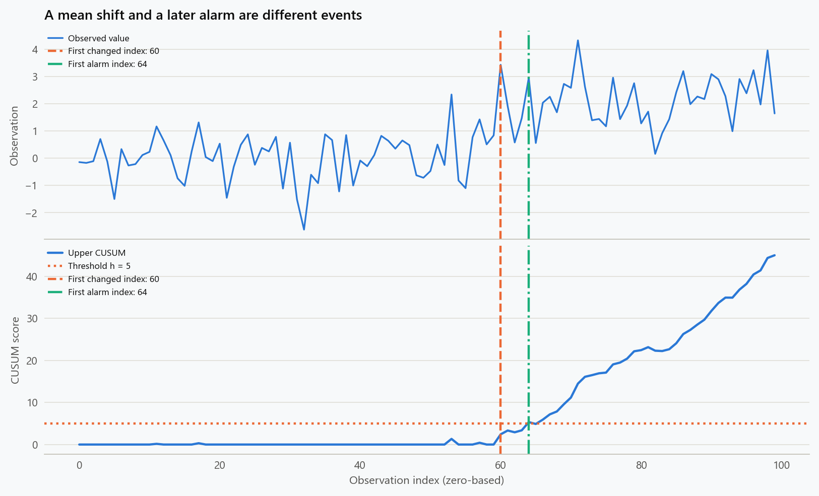
Original synthetic example. The first alarm and the known simulated change are marked separately. The threshold is not calibrated to a claimed false-alarm rate.

The numerical model, reproducibility tests, and figure renderer are maintained in the blog-reproducibility repository. The CUSUM figure script reproduces this example; run it with --dry-run to print the observations, scores, and alarm index without writing an image.

Check the Implementation Against the Definition

For a supplied finite series, independently calculate every suffix sum of $X_t-\mu_0-\delta/2$, include the empty sum, and take the maximum. At each time, that exhaustive calculation must agree with the recursive score. This is a stronger check than asserting that one simulation produces a plausible-looking alarm.

Other useful cases include an empty series, a first-observation alarm, a series that never alarms, and a score exactly equal to the threshold. The last case checks the strict > rule. Shifting both the observations and baseline by the same constant should leave the scores unchanged. Multiplying observations, baseline, target shift, and threshold by the same positive factor should preserve the alarm index while scaling the scores.

These checks establish implementation consistency with the specified statistic. They do not establish its fitness for a particular monitoring application. That final claim requires evidence about the data-generating process, the consequences of false alarms and delays, and the complete policy that surrounds the detector.