Topics
Sequential change-point detection watches a stream and raises an alarm as soon as it is confident something has changed. It trades detection delay against false alarms, and it is the right tool for monitoring. The retrospective question is different. Two years of a sensor's history are on disk, the baseline appears to have stepped several times, and the questions are where and how many. A process yield shifted after each of a series of undocumented interventions, and the maintenance log needs reconstructing. That is offline change-point detection, and it is a partition problem: cut the series into segments so that each is homogeneous, paying a price for every cut.
The Problem as a Penalised Partition
Given a series $x_1, \dots, x_n$ and a cost $C(\cdot)$ that measures how badly a segment fits a single model, the offline problem is
with $\tau_0 = 0$ and $\tau_{k+1} = n$. For changes in mean the natural cost is the sum of squared deviations from the segment mean; for changes in variance or in a regression slope it is the corresponding negative log-likelihood. The penalty $\beta$ per change point is what stops the solution from placing a cut between every pair of points.
The minimum over all partitions looks like a combinatorial search and is not. Because the cost is additive over segments, the best partition of the first $b$ points is the best partition of the first $a$ points plus one final segment, for the best choice of $a$, and that recursion solves the problem exactly in $O(n^2)$. This is optimal partitioning; PELT, from Killick, Fearnhead and Eckley, prunes candidate $a$ values that can never win and runs in close to linear time. Binary segmentation, the older alternative, finds the single best cut, then the best cut in each half, and so on; it is fast and greedy, and it can miss changes that are only visible once their neighbours have been found.
An Exact Implementation
1
2
3
4
5
6
7
8
9
10
11
12
13
14
15
16
17
18
19
20
21
22
23
24
25
26
27
28
29
30
31
32
33
34
35
36
37
38
39
40
41
42
43
44
45
46
47
48
49
50
51
import numpy as np

def make_series(r, n=600, phi=0.0):
    bounds = [0, 120, 200, 350, 420, 600]
    means = [0.0, 1.5, 0.0, -1.2, 1.0]
    mu = np.zeros(n)
    for (a, b), m in zip(zip(bounds[:-1], bounds[1:]), means):
        mu[a:b] = m
    e = r.normal(size=n)
    if phi:                                          # optional AR(1) noise
        for t in range(1, n):
            e[t] = phi * e[t-1] + np.sqrt(1 - phi**2) * e[t]
    return mu + e, bounds[1:-1]

def optimal_partition(x, penalty):
    """Exact minimisation of sum of squared residuals + penalty per change point, O(n^2)."""
    n = len(x)
    cs, cs2 = np.concatenate([[0.0], np.cumsum(x)]), np.concatenate([[0.0], np.cumsum(x**2)])
    def cost(a, b):                                  # RSS of segment x[a:b]
        s, s2 = cs[b] - cs[a], cs2[b] - cs2[a]
        return s2 - s * s / (b - a)
    F = np.full(n + 1, np.inf); F[0] = -penalty
    last = np.zeros(n + 1, dtype=int)
    for b in range(1, n + 1):
        cands = [F[a] + cost(a, b) + penalty for a in range(b)]
        a = int(np.argmin(cands)); F[b] = cands[a]; last[b] = a
    cps, b = [], n
    while last[b] > 0:
        cps.append(int(last[b])); b = last[b]
    return sorted(cps)

def robust_sigma(x):
    d = np.diff(x)
    return np.median(np.abs(d - np.median(d))) / 0.6745 / np.sqrt(2)

def score(found, true, tol=5):
    tp = sum(any(abs(f - t) <= tol for t in true) for f in found)
    prec = tp / len(found) if found else 1.0
    rec = sum(any(abs(f - t) <= tol for f in found) for t in true) / len(true)
    return prec, rec

r = np.random.default_rng(0)
x, true_cps = make_series(r)
n = len(x)
sig = robust_sigma(x)
print(f"true change points: {true_cps}; robust sigma estimate {sig:.2f} (sample sd {x.std():.2f})")
print("penalty multiple of log n   change points found                    precision  recall")
for mult in (0.5, 1, 2, 4, 8):
    cps = optimal_partition(x, mult * np.log(n) * sig**2)
    p, rc = score(cps, true_cps)
    print(f"{mult:<27}{str(cps) if len(cps) < 12 else str(len(cps)) + ' found':<40}{p:>8.2f}{rc:>8.2f}")
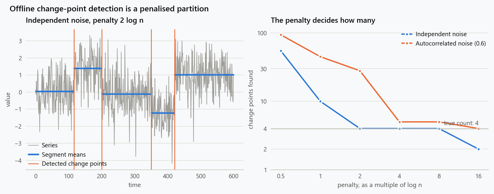
The series has 600 points, four shifts in mean of between 1.2 and 2.2 noise standard deviations, and unit noise. The penalty is expressed as a multiple of $\sigma^2 \log n$, the scale at which the Schwarz criterion places it.
| Penalty, multiples of $\sigma^2 \log n$ | Change points found | Precision | Recall |
|---|---|---|---|
| 0.5 | 55 | 0.13 | 1.00 |
| 1 | 10 | 0.40 | 1.00 |
| 2 | 116, 200, 350, 421 | 1.00 | 1.00 |
| 4 | 116, 200, 350, 421 | 1.00 | 1.00 |
| 8 | 116, 200, 350, 421 | 1.00 | 1.00 |
The true change points are at 120, 200, 350 and 420. With a penalty at twice the Schwarz scale and above, the partition finds exactly four, within a few points of the truth. With the penalty halved it finds fifty-five, every one of them a place where the noise happened to dip or rise for a few samples. The algorithm did not change; the price of a cut did. The number of change points in a series is not a fact the method discovers. It is a consequence of the penalty, and the penalty is a decision.
Choosing the Penalty
Two things go into a defensible penalty: a scale, and a noise level to multiply it by.
The scale comes from information criteria. For a change in mean with known noise variance, Yao showed that a penalty proportional to $\log n$ per change point recovers the true number of changes as the series grows, and $2\sigma^2 \log n$ is the common default. The table shows why the exact multiple matters less than it seems: the count is four from two times the scale to eight times it. A plateau in the count across a range of penalties is the signature of a real set of changes, and a count that slides continuously with the penalty is the signature of noise being partitioned.
The cost-against-count curve says the same thing from the other side.
1
2
3
4
5
6
7
8
9
seen = {}
for pen in np.exp(np.linspace(np.log(2), np.log(400), 60)):
    cps = optimal_partition(x, pen)
    k = len(cps)
    if k not in seen:
        b = [0] + cps + [n]
        seen[k] = sum(((x[a:c] - x[a:c].mean())**2).sum() for a, c in zip(b[:-1], b[1:]))
for k in sorted(seen)[:6]:
    print(f"  k = {k:>2}: RSS {seen[k]:7.1f}")
| Change points | Residual sum of squares |
|---|---|
| 0 | 978 |
| 2 | 723 |
| 3 | 647 |
| 4 | 588 |
| 6 | 571 |
| 10 | 544 |
Each of the first four cuts removes between about 60 and 130 units of cost. The fifth and sixth together remove 17, and each cut after that removes about what a cut placed at random in pure noise would. The elbow is at four, and it is the same answer the penalty plateau gave.
The noise level is the input people forget. The penalty is $\beta \sigma^2$, and $\sigma$ has to be estimated from a series that contains the very shifts being looked for. The sample standard deviation of this series is 1.28, because it includes the shifts; the noise is 1. The estimator in the code uses the median absolute deviation of first differences, which the shifts barely touch, and returns 0.96. Here the shifts are large enough that the inflated estimate still finds all four. With subtler shifts, an inflated $\sigma$ raises the penalty by the square of the inflation and hides them.
Autocorrelation Makes Everything Look Like a Change
Almost every industrial series is autocorrelated: a temperature, a vibration level or a yield does not reset to independence between samples. That breaks the noise assumption behind the penalty in a specific and severe way.
1
2
3
4
5
6
7
xa, _ = make_series(np.random.default_rng(1), phi=0.6)
siga = robust_sigma(xa)
for mult in (2, 4, 8, 16):
    cps = optimal_partition(xa, mult * np.log(n) * siga**2)
    p, rc = score(cps, true_cps)
    print(f"  penalty {mult:>2} log n: {len(cps):>2} change points, precision {p:.2f}, recall {rc:.2f}")
print(f"  long-run variance factor (1+phi)/(1-phi) = {(1+0.6)/(1-0.6):.1f}; robust sigma on the AR series {siga:.2f}")
| Penalty, multiples of $\hat\sigma^2 \log n$ | Change points found | Precision | Recall |
|---|---|---|---|
| 2 | 28 | 0.11 | 0.75 |
| 4 | 5 | 0.80 | 1.00 |
| 8 | 5 | 0.80 | 1.00 |
| 16 | 4 | 0.75 | 0.75 |
Same four shifts, noise with an autocorrelation of 0.6 at lag one. The default penalty finds twenty-eight change points, of which three are real. Autocorrelated noise wanders: it stays above its mean for a run of samples and then below, and every such run looks to a squared-error cost like a segment with a different mean.
Two things compound. The variance that matters for a segment mean is the long-run variance, which for this process is $(1 + \phi)/(1 - \phi) = 4$ times the marginal variance. And the robust estimator is fooled in the other direction: first differences of an autocorrelated series are smaller than the marginal noise, by a factor of $\sqrt{1 - \phi}$, so it returns 0.63 for a process whose marginal standard deviation is one. The penalty is therefore too small by a factor of about ten, and the twenty-eight change points follow.
Scaling the penalty by the long-run variance factor brings the count to five, with all four true changes found and one spurious. Over 200 replications, the default penalty on independent noise gives a precision and recall of 0.95 and finds 4.1 change points on average; on the autocorrelated series it gives a precision of 0.13 and finds 29.5. The remedies are to estimate the long-run variance and inflate the penalty by it, to fit an autoregressive model and segment its residuals, or to segment block averages at a resolution coarse enough that the blocks are close to independent. What is not a remedy is the library default.
Reading the Result
Locations have uncertainty. The first change is found at 116 against a true 120, because the noise around the boundary makes a cut four samples early fit slightly better. A tolerance of a few samples is part of any honest scoring, and a change point reported to the sample is over-precise.
Short segments are suspect. A segment of six samples between two cuts is more often two cuts around a noise excursion than a real regime. A minimum segment length, enforced in the recursion by restricting the candidates for $a$, removes most of them and is standard in the libraries.
The cost defines the change. A squared-error cost on the level sees a change in slope as a staircase of small mean shifts, and a change in variance not at all. A series that ramps needs a cost built on a linear fit within each segment; a series whose noise changes needs one built on the variance. The method is the same; the cost has to match the kind of change being looked for.
Multivariate series are handled by summing the cost across channels, which detects changes that are shared, or by segmenting channels separately, which detects changes that are not. Which is wanted depends on whether a single event is being reconstructed or each channel's own history.
Offline and Sequential
The two problems share cost functions and little else. The sequential detector's obligation is speed under a false-alarm constraint, and it cannot use data from after the change. The offline method uses everything and has no delay to trade, so it locates changes more precisely and counts them more reliably, and its false alarms are controlled by the penalty rather than by a threshold. In a monitoring system the two are complementary: the offline segmentation of the history is how the regimes are labeled, how the sequential detector's threshold is tuned, and how its past alarms are audited.
What to Do
- Choose the cost for the change expected: level, slope, variance or distribution.
- Estimate the noise scale robustly, and if the series is autocorrelated, inflate it by the long-run variance factor or segment residuals from a fitted model.
- Sweep the penalty and plot the count of change points against it, and the cost against the count. A plateau and an elbow that agree are the answer; a count that slides with the penalty is noise.
- Enforce a minimum segment length consistent with the shortest regime that could be real.
- Validate by simulation on a series with the same noise structure and no changes, and confirm that the chosen penalty finds none.
- Report locations with a tolerance, and the penalty that produced them.
The figure generator in the blog-reproducibility repository reproduces this article's figure; run it with --dry-run to print the numbers behind the figure without writing an image.
References
- Killick, R., Fearnhead, P., & Eckley, I. A. (2012). Optimal detection of changepoints with a linear computational cost. Journal of the American Statistical Association, 107(500), 1590-1598.
- Jackson, B., Scargle, J. D., Barnes, D., Arabhi, S., Alt, A., Gioumousis, P., Gwin, E., Sangtrakulcharoen, P., Tan, L., & Tsai, T. T. (2005). An algorithm for optimal partitioning of data on an interval. IEEE Signal Processing Letters, 12(2), 105-108.
- Yao, Y.-C. (1988). Estimating the number of change-points via Schwarz' criterion. Statistics and Probability Letters, 6(3), 181-189.
- Scott, A. J., & Knott, M. (1974). A cluster analysis method for grouping means in the analysis of variance. Biometrics, 30(3), 507-512.
- Fryzlewicz, P. (2014). Wild binary segmentation for multiple change-point detection. The Annals of Statistics, 42(6), 2243-2281.
- Truong, C., Oudre, L., & Vayatis, N. (2020). Selective review of offline change point detection methods. Signal Processing, 167, 107299.
Embed interactive plots, widgets, and demos using <figure>, <iframe>, or <div class="interactive-embed"> containers. Ensure each embed includes descriptive captions for accessibility.
How to cite
Use the quick export buttons to save citations for reference managers or copy the formatted text directly.
Diogo Ribeiro (2025). Offline Change-Point Detection: Segmenting a Series After the Fact. Faculty of Media Arts and Design, Technical University of Porto. https://diogoribeiro7.github.io/time-series/offline_change_point_detection_segmentation/.


