Unequal Allocation: What a Ninety-Ten Split Costs

The rollout plan sends ten percent of traffic to the new version. It is the cautious choice, it limits the blast radius, and everybody signs it. Then the experiment runs for three weeks instead of one, and the result is still ambiguous.

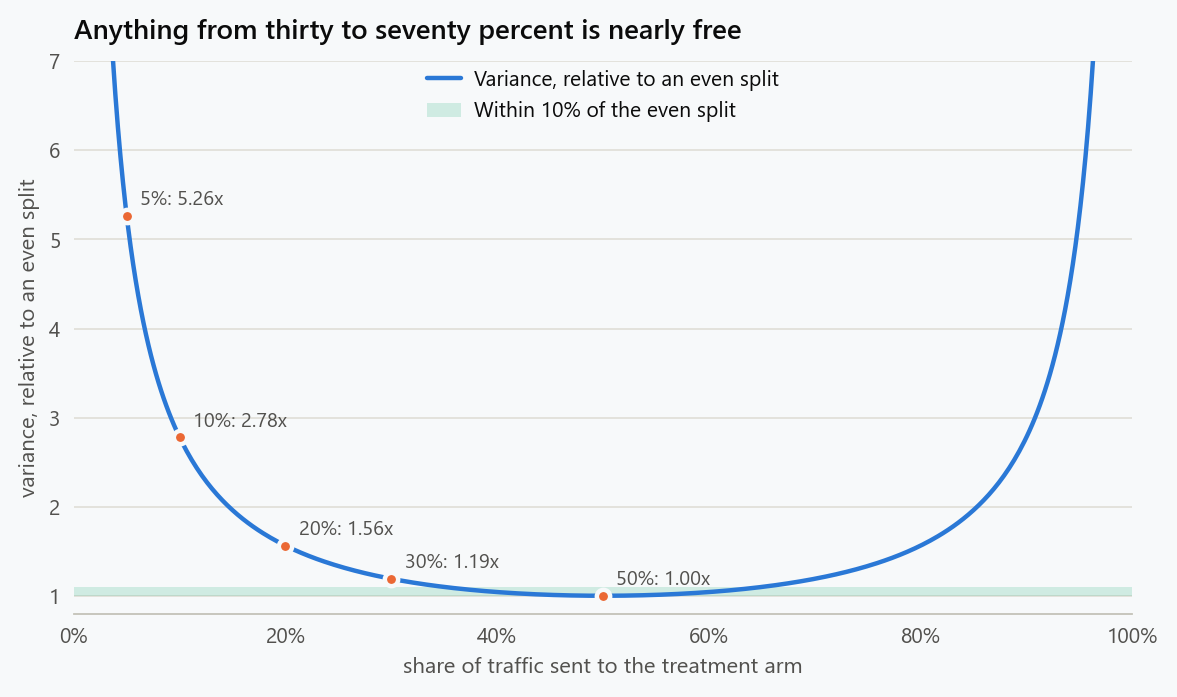
Both facts follow from one formula. The precision of a comparison depends on the product of the two arm shares, so a ninety-ten split carries 2.8 times the variance of an even one. The caution is not free, its price is computable before the test starts, and it is often worth paying. What is not defensible is paying it without knowing the amount.

Where the Cost Comes From

With a total of <div class="math-expression math-expression--source" data-math-alt="N" data-math-source="N" aria-label="N" tabindex="0">\(N\)</div> users and a fraction <div class="math-expression math-expression--source" data-math-alt="f" data-math-source="f" aria-label="f" tabindex="0">\(f\)</div> in the treatment arm, the variance of the difference in means is

The product <div class="math-expression math-expression--source" data-math-alt="f(1-f)" data-math-source="f(1-f)" aria-label="f(1-f)" tabindex="0">\(f(1-f)\)</div> is maximised at a half and falls away sharply, so relative to an even split the variance is inflated by <div class="math-expression math-expression--source" data-math-alt="0.25 / (f(1-f))" data-math-source="0.25 / (f(1-f))" aria-label="0.25 / (f(1-f))" tabindex="0">\(0.25 / (f(1-f))\)</div>.

1
2
3
4
5
6
7
8
9
10
11
12
13
14
15
16
17
18
19
20
21
22
23
24
25
26
27
import numpy as np
from scipy import stats

RNG = np.random.default_rng(53)
ZC = stats.norm.ppf(0.975)
ZB = stats.norm.ppf(0.80)


def variance_factor(f):
    """Variance of the difference in means, relative to an even split."""
    return 0.25 / (f * (1 - f))


def power_at(n_total, f, delta, sd):
    se = sd * np.sqrt(1 / (f * n_total) + 1 / ((1 - f) * n_total))
    z = delta / se
    return stats.norm.cdf(z - ZC) + stats.norm.cdf(-ZC - z)


DELTA, SD, N = 0.02, 0.45, 40000
for f in (0.5, 0.4, 0.3, 0.2, 0.1, 0.05):
    factor = variance_factor(f)
    print(f"{f:4.0%} to treatment: variance {factor:5.2f}x, "
          f"users needed for the same power {factor:5.2f}x, "
          f"power at {N:,} users {power_at(N, f, DELTA, SD):5.1%}, "
          f"smallest detectable effect "
          f"{(ZC + ZB) * SD * np.sqrt(1 / (f * N) + 1 / ((1 - f) * N)):.4f}")

The shape of that column is the useful thing to remember. Anything from 40 to 60 percent is free: a 60/40 split costs four percent more traffic, which nobody will notice. Below about 25 percent the cost climbs steeply, and by five percent the test needs more than five times the users.

1
2
3
4
5
6
7
8
9
10
11
12
for f in (0.5, 0.3, 0.1):
    hits = 0
    reps = 4000
    for _ in range(reps):
        nt = int(round(f * N))
        nc = N - nt
        t = RNG.normal(DELTA, SD, nt)
        c = RNG.normal(0.0, SD, nc)
        se = np.sqrt(t.var(ddof=1) / nt + c.var(ddof=1) / nc)
        hits += abs(t.mean() - c.mean()) / se > ZC
    print(f"{f:4.0%} to treatment: formula {power_at(N, f, DELTA, SD):5.1%}, "
          f"simulated {hits / reps:5.1%}")

The Price of Caution, in Days

Traffic arrives at a rate, so the honest unit for this cost is time.

1
2
3
4
5
DAILY = 2000
for f in (0.5, 0.25, 0.10, 0.05, 0.01):
    n_needed = 2 * (ZC + ZB) ** 2 * SD ** 2 / DELTA ** 2 * variance_factor(f) * 2
    print(f"{f:4.0%} to treatment: {n_needed:11,.0f} users for 80% power, "
          f"{n_needed / DAILY:6.1f} days at {DAILY:,} users a day")

A one percent exposure is not a cautious experiment, it is a two-hundred-day experiment, which in practice means an experiment that never concludes and a decision made on something else. If the risk genuinely requires a one percent exposure, the honest plan is a staged rollout with safety monitoring rather than a test sized to measure a two percent effect.

When Uneven Is Right: Different Spread

Even allocation is optimal when the arms have equal variance. When they do not, precision improves by putting more users where the variability is, which is Neyman allocation: <div class="math-expression math-expression--source" data-math-alt="f^ = _t / ( _t + _c)" data-math-source="f^\star = \sigma_t / (\sigma_t + \sigma_c)" aria-label="f^ = _t / ( _t + _c)" tabindex="0">\(f^\star = \sigma_t / (\sigma_t + \sigma_c)\)</div>.

1
2
3
4
5
6
7
8
9
10
11
12
def optimal_f(sd_t, sd_c):
    """Neyman allocation: put people where the variance is."""
    return sd_t / (sd_t + sd_c)


for sd_t, sd_c in ((0.45, 0.45), (0.60, 0.30), (0.90, 0.30), (0.30, 0.90)):
    f_star = optimal_f(sd_t, sd_c)
    var_even = sd_t ** 2 / (0.5 * N) + sd_c ** 2 / (0.5 * N)
    var_star = sd_t ** 2 / (f_star * N) + sd_c ** 2 / ((1 - f_star) * N)
    print(f"spread {sd_t:.2f} against {sd_c:.2f}: best split {f_star:4.0%} to treatment, "
          f"variance {var_star / var_even:5.3f}x the even split, "
          f"users saved {1 - var_star / var_even:5.1%}")

A treatment that triples the spread of the outcome, which happens when a feature helps some users a great deal and others not at all, is worth 75 percent of the traffic, and the saving is a fifth of the sample. This is the one case where the optimum is meaningfully uneven for statistical rather than practical reasons, and it is also the case teams least expect, because the instinct is to protect users from the new thing rather than to measure it more closely.

When Uneven Is Right: Different Cost

If one arm costs more per user, in compute, in support load or in discount given away, the budget buys more precision when the expensive arm is smaller. Minimising variance for a fixed budget puts a share <div class="math-expression math-expression--source" data-math-alt="1/(1+square root of c)" data-math-source="1/(1+\sqrt{c})" aria-label="1/(1+square root of c)" tabindex="0">\(1/(1+\sqrt{c})\)</div> in the arm that costs <div class="math-expression math-expression--source" data-math-alt="c" data-math-source="c" aria-label="c" tabindex="0">\(c\)</div> times as much.

1
2
3
4
5
6
7
8
9
10
11
12
for cost_ratio in (1, 2, 4, 10):
    # Minimising variance for a fixed budget puts fewer users where they cost more.
    f_star = 1 / (1 + np.sqrt(cost_ratio))
    budget = N * (1 + 1) / 2            # budget of an even split at cost 1 each
    # Users affordable at this split, given the treatment costs `cost_ratio`.
    scale = budget / (f_star * cost_ratio + (1 - f_star))
    var_star = SD ** 2 * (1 / (f_star * scale) + 1 / ((1 - f_star) * scale))
    even_scale = budget / (0.5 * cost_ratio + 0.5)
    var_even = SD ** 2 * (1 / (0.5 * even_scale) + 1 / (0.5 * even_scale))
    print(f"treatment costs {cost_ratio:2d}x: best split {f_star:4.0%} to treatment, "
          f"{scale:8,.0f} users affordable, variance {var_star / var_even:5.3f}x "
          f"the even split on the same budget")

The gains are modest, three to twenty percent, which is worth knowing in both directions: tilting the split for cost is a real improvement, and it is not a large one. A treatment ten times as expensive still deserves a quarter of the users, not five percent.

When Uneven Is Right: One Control, Several Treatments

The clearest case is the most common one. When several variants are compared against a single control, every comparison uses that control, so it should be larger than each treatment. The optimum allocates the control in proportion to the square root of the number of treatment arms.

1
2
3
4
5
6
7
8
9
10
11
12
for k in (1, 2, 3, 5, 8):
    # Equal split across all arms, against the square-root rule for the control.
    f_control_equal = 1 / (k + 1)
    f_control_sqrt = np.sqrt(k) / (np.sqrt(k) + k)
    def var_one(fc):
        ft = (1 - fc) / k
        return SD ** 2 * (1 / (ft * N) + 1 / (fc * N))
    print(f"{k} treatment arm(s): equal split gives control {f_control_equal:4.0%} "
          f"and variance {var_one(f_control_equal):.3e}; "
          f"square-root rule gives control {f_control_sqrt:4.0%} "
          f"and variance {var_one(f_control_sqrt):.3e}, "
          f"{1 - var_one(f_control_sqrt) / var_one(f_control_equal):5.1%} lower")

With eight variants the usual equal split gives the control eleven percent of traffic and every comparison inherits that thin baseline. Giving the control 26 percent cuts the variance of each comparison by nearly a fifth, for free, by moving users between arms rather than adding any.

What to Do

1. Compute the inflation factor before agreeing a split. One over four times the product of the two shares, relative to an even split, is the whole formula.
2. Treat anything between 40 and 60 percent as free and anything below 25 percent as a decision with a price in days.
3. When the exposure has to be small for safety, stage the rollout and monitor for harm instead of pretending a one percent test will measure a small effect.
4. Allocate more to the arm with more spread when the variances differ. A treatment that widens the outcome distribution deserves more users, not fewer.
5. Give a shared control the square root of the number of treatment arms. With five or more variants this is the cheapest precision available.
6. Recompute the duration after fixing the split, and put the result in the test plan. Most disagreements about traffic splits end when the cost is quoted in days.

References

• Neyman, J. (1934). On the two different aspects of the representative method. Journal of the Royal Statistical Society, 97(4), 558-625.
• Dunnett, C. W. (1955). A multiple comparison procedure for comparing several treatments with a control. Journal of the American Statistical Association, 50(272), 1096-1121.
• Pocock, S. J. (1983). Clinical Trials: A Practical Approach. Wiley.
• Hu, F., & Rosenberger, W. F. (2006). The Theory of Response-Adaptive Randomization in Clinical Trials. Wiley.
• Kohavi, R., Tang, D., & Xu, Y. (2020). Trustworthy Online Controlled Experiments: A Practical Guide to A/B Testing. Cambridge University Press.
• Deng, A., Li, Y., Lu, J., & Ramamurthy, V. (2021). On post-selection inference in A/B testing. Proceedings of the 27th ACM SIGKDD Conference on Knowledge Discovery and Data Mining, 2743-2752.