Topics
The team rebuilt the saved-items panel, ran the experiment on the whole user base for three weeks, and read a 0.6 percent lift in revenue per user with a confidence interval straddling zero. The verdict was recorded as no effect. Eight percent of users open that panel in a given month. Among those users the change was worth 6 percent, which is one of the largest wins the team shipped that year, and the experiment could not see it because 92 percent of the measurement was made on people for whom the feature did not exist.
This is dilution, and it is arithmetic rather than misfortune. If an effect exists only among the fraction $p$ of users who reach a feature, the effect on the whole population is $p$ times as large. The dashboard is not wrong. It is answering a question about the population when the decision needs an answer about the feature.
A Population in Two Parts
The simulation splits users into those who reach the feature and those who never do. The first group is more active and more variable, which is the usual situation: people who open a panel are people who use the product. The treatment raises the triggered users' outcome by 6 percent and leaves everyone else untouched.
1
2
3
4
5
6
7
8
9
10
11
12
13
14
15
16
17
18
19
20
21
22
23
24
25
26
27
28
29
30
31
32
33
34
35
36
import numpy as np
from scipy import stats

RNG = np.random.default_rng(3)

MU_NON, SD_NON = 18.0, 9.0     # users who never reach the feature
MU_TRIG, SD_TRIG = 30.0, 14.0  # users who do: more active, more variable
LIFT = 0.06                    # the feature's effect on the users who see it
TRUTH = MU_TRIG * LIFT         # 1.80, the effect on a triggered user


def arm(n, p, treated, lift=LIFT, rng=RNG):
    """One arm: outcomes and trigger flags for n users with trigger rate p."""
    trig = rng.random(n) < p
    y = np.where(trig, rng.normal(MU_TRIG, SD_TRIG, n), rng.normal(MU_NON, SD_NON, n))
    if treated:
        y = np.where(trig, y * (1 + lift), y)
    return y, trig


def welch(a, b):
    """Difference in means, its standard error and the two-sided p-value."""
    d = b.mean() - a.mean()
    se = np.sqrt(a.var(ddof=1) / a.size + b.var(ddof=1) / b.size)
    return d, se, 2 * (1 - stats.norm.cdf(abs(d / se)))


print(f"true effect on a triggered user: {TRUTH:.3f} ({LIFT:.0%} of {MU_TRIG:.0f})")
for p in (0.50, 0.20, 0.08, 0.02):
    yc, tc = arm(200_000, p, False)
    yt, tt = arm(200_000, p, True)
    d_all, se_all, p_all = welch(yc, yt)
    d_tr, se_tr, p_tr = welch(yc[tc], yt[tt])
    print(f"trigger rate {p:5.0%}: all users {d_all:+6.3f} (se {se_all:.3f}, p {p_all:6.3f})"
          f"   triggered only {d_tr:+6.3f} (se {se_tr:.3f}, p {p_tr:6.3f})"
          f"   dilution predicts {p * TRUTH:+6.3f}")
| Trigger rate | All users | Standard error | Triggered only | Standard error | Dilution predicts |
|---|---|---|---|---|---|
| 50% | +0.893 | 0.043 | +1.730 | 0.064 | +0.900 |
| 20% | +0.343 | 0.036 | +1.716 | 0.102 | +0.360 |
| 8% | +0.204 | 0.032 | +1.963 | 0.161 | +0.144 |
| 2% | +0.070 | 0.029 | +1.897 | 0.322 | +0.036 |
The triggered-only estimate recovers the 1.80 truth at every trigger rate, with a standard error that widens as the triggered group shrinks. The all-user estimate tracks $p \times 1.80$, as predicted, and at a 2 percent trigger rate it has shrunk to 0.070 against a standard error of 0.029, which is on the edge of visibility with 200,000 users per arm.
What Dilution Costs in Traffic
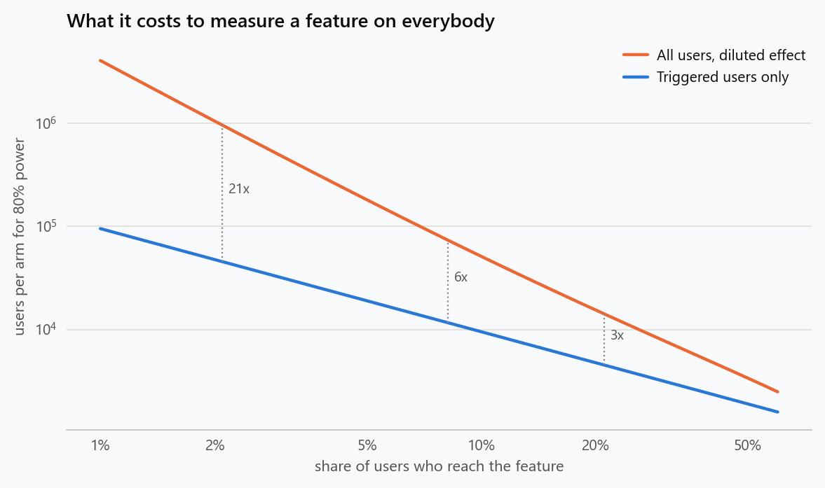
The sample size for a fixed power follows from the two ingredients: the effect the analysis is looking at, and the variance of the metric it is looking at. Diluting the effect by $p$ divides the numerator by $p^2$ in the sample size formula. Restricting to triggered users restores the full effect but throws away all the non-triggered users, so the users needed scale as $1/p$ rather than $1/p^2$.
1
2
3
4
5
6
7
8
9
10
11
12
13
14
15
16
17
18
19
20
21
22
23
24
25
26
27
28
29
30
31
32
ZS = (stats.norm.ppf(0.975) + stats.norm.ppf(0.8)) ** 2


def var_all(p):
    """Variance of the outcome over the whole population at trigger rate p."""
    m = p * MU_TRIG + (1 - p) * MU_NON
    return (p * (SD_TRIG ** 2 + MU_TRIG ** 2)
            + (1 - p) * (SD_NON ** 2 + MU_NON ** 2) - m ** 2)


sizes = {}
for p in (0.50, 0.20, 0.08, 0.02):
    n_all = 2 * var_all(p) * ZS / (p * TRUTH) ** 2
    n_trig = 2 * SD_TRIG ** 2 * ZS / TRUTH ** 2 / p
    sizes[p] = (n_all, n_trig)
    print(f"trigger rate {p:5.0%}: all users {n_all:12,.0f}   "
          f"triggered only {n_trig:11,.0f}   ratio {n_all / n_trig:6.1f}x")

for p in (0.20, 0.08):
    for label, n, triggered in (("all users", sizes[p][0], False),
                                ("triggered only", sizes[p][1], True)):
        n = int(round(n))
        r = np.random.default_rng(101)
        hits = 0
        for _ in range(500):
            yc, tc = arm(n, p, False, rng=r)
            yt, tt = arm(n, p, True, rng=r)
            if triggered:
                hits += welch(yc[tc], yt[tt])[2] < 0.05
            else:
                hits += welch(yc, yt)[2] < 0.05
        print(f"trigger rate {p:4.0%}, {label:15s} {n:9,} users per arm: power {hits / 500:5.1%}")
| Trigger rate | Users per arm, all users | Users per arm, triggered only | Ratio | Measured power |
|---|---|---|---|---|
| 50% | 3,382 | 1,899 | 1.8x | — |
| 20% | 15,388 | 4,748 | 3.2x | 78.8% and 79.8% |
| 8% | 76,307 | 11,870 | 6.4x | 79.2% and 77.4% |
| 2% | 1,043,155 | 47,481 | 22.0x | — |
Both closed forms are right: run at exactly the predicted size, the simulated power lands between 77 and 80 percent in all four cases. The ratio column is the cost of the diluted analysis. At a 20 percent trigger rate it is three times the traffic; at 2 percent it is twenty-two times, which turns a two-week test into a year.
The ratio is not simply $1/p$ because the two analyses look at different variances. The triggered population is more variable in absolute terms, which works against it, while the whole population is dominated by the quieter non-triggered users, which works in its favour. The first effect is much smaller than the dilution, so the triggered analysis wins by a wide margin whenever the trigger rate is low.
When the Triggered Analysis Breaks
The triggered analysis looks like a free win, and it usually is. It has one requirement: triggering must not itself be affected by the treatment. When the treatment changes who triggers, the two triggered groups are no longer the same kind of user, and comparing them compares populations rather than versions.
Suppose the new panel is easier to find, so the treatment pulls in users further down the activity distribution who would not have opened the old one. The simulation gives the treatment an extra slice of the population and then estimates the effect three ways: on the users who triggered as logged, on the users who would have triggered under control, and on everyone.
1
2
3
4
5
6
7
8
9
10
11
12
13
14
15
16
17
18
19
20
21
22
23
24
25
26
27
28
29
def composition(n, p, extra, lift=LIFT, rng=RNG):
    """Treatment reaches `extra` more of the population, lower down the activity scale."""
    out = []
    for treated in (False, True):
        activity = rng.normal(0, 1, n)
        cut = stats.norm.ppf(1 - p)                    # who the feature reaches in control
        cut_t = stats.norm.ppf(1 - p - extra)          # and in treatment
        trig = activity > (cut_t if treated else cut)
        y = np.where(activity > cut,
                     rng.normal(MU_TRIG, SD_TRIG, n),
                     rng.normal(MU_NON, SD_NON, n))
        if treated:
            y = np.where(trig, y * (1 + lift), y)
        out.append((y, trig, activity > cut))
    return out


for extra in (0.00, 0.04, 0.10):
    logged, counter, everyone = [], [], []
    r = np.random.default_rng(5)
    for _ in range(20):
        (yc, tc, ec), (yt, tt, et) = composition(200_000, 0.08, extra, rng=r)
        logged.append(yt[tt].mean() - yc[tc].mean())
        counter.append(yt[et].mean() - yc[ec].mean())
        everyone.append(yt.mean() - yc.mean())
    print(f"treatment widens the trigger by {extra:4.0%} of users: "
          f"triggered as logged {np.mean(logged):+6.3f}   "
          f"counterfactual trigger {np.mean(counter):+6.3f}   "
          f"all users {np.mean(everyone):+6.3f}   (truth on the original group {TRUTH:+.3f})")
| Treatment widens the trigger by | Triggered as logged | Counterfactual trigger | All users |
|---|---|---|---|
| 0% of users | +1.888 | +1.888 | +0.142 |
| 4% of users | −2.371 | +1.888 | +0.185 |
| 10% of users | −5.224 | +1.888 | +0.250 |
With no change in triggering, the logged and counterfactual analyses agree and both recover the 1.80 truth. As soon as the treatment widens the trigger, the logged analysis collapses and then reverses sign: a feature worth plus 6 percent is measured at minus 8 percent and then minus 17 percent. The mechanism is not subtle. The treatment's triggered group now contains users whose outcome averages 18, the control's contains only users averaging 30, and the difference between those populations swamps the effect.
The counterfactual analysis is immune because it defines the triggered set the same way in both arms, from information that predates the assignment. The all-user estimate also stays interpretable, and it even grows, which is correct: reaching more users with a positive feature is a real gain.
Which Question the Decision Needs
Dilution is a measurement problem; it is not always a problem with the metric. The all-user number is the right one for a forecast, because the company's revenue is the population number and not the triggered number. The triggered number is the right one for a decision about the feature, because it measures what the change does when it is used, and it is the number that generalises if the feature is later made easier to find.
The practical consequence is that both belong in the report. A feature with a 6 percent effect on 8 percent of users is worth 0.76 percent overall today, and might be worth 2 percent if the entry point moves. Reporting only the diluted figure hides the feature's quality; reporting only the triggered figure overstates its value to the business.
1
2
3
4
5
6
for p in (0.50, 0.20, 0.08, 0.02):
    mean_all = p * MU_TRIG + (1 - p) * MU_NON
    mde = np.sqrt(2 * var_all(p) / 200_000) * (stats.norm.ppf(0.975) + stats.norm.ppf(0.8))
    print(f"trigger rate {p:5.0%}: diluted effect {p * TRUTH / mean_all:6.2%} of the metric, "
          f"smallest detectable {mde / mean_all:6.2%}, "
          f"{'visible' if p * TRUTH > mde else 'invisible':>9s}")
| Trigger rate | Diluted effect on the metric | Smallest effect visible with 200,000 per arm | Verdict |
|---|---|---|---|
| 50% | 3.75% | 0.49% | visible |
| 20% | 1.76% | 0.49% | visible |
| 8% | 0.76% | 0.47% | visible |
| 2% | 0.20% | 0.45% | invisible |
The last row is the one that produces false conclusions. A real 6 percent improvement to a feature used by one user in fifty is invisible at 200,000 users per arm, and the experiment will report no effect with a straight face. Knowing the trigger rate in advance is what separates "no effect" from "no power".
What to Do
- Record the trigger rate before the test starts, from historical logs. It determines the sample size and whether the question is answerable at all.
- Log the trigger condition in both arms, evaluated the same way, using information available before the assignment took effect. This is the single change that makes a triggered analysis trustworthy.
- Check that the trigger rate is equal across arms before reading a triggered result. A difference is evidence that the treatment moved the trigger, and the triggered comparison is then between different populations.
- Report the triggered effect and the diluted effect together, with the trigger rate that connects them.
- Size on the analysis you will act on. A triggered analysis needs users in proportion to one over the trigger rate; an all-user analysis needs one over its square.
- When the trigger cannot be logged counterfactually, keep the all-user estimate as the primary result and treat the triggered figure as an upper bound.
The figure generator in the blog-reproducibility repository reproduces this article's figure; run it with --dry-run to print the numbers behind the figure without writing an image.
References
- Deng, A., Lu, J., & Litz, J. (2017). Trustworthy analysis of online A/B tests: pitfalls, challenges and solutions. Proceedings of the Tenth ACM International Conference on Web Search and Data Mining, 641-649.
- Kohavi, R., Deng, A., Frasca, B., Walker, T., Xu, Y., & Pohlmann, N. (2013). Online controlled experiments at large scale. Proceedings of the 19th ACM SIGKDD International Conference on Knowledge Discovery and Data Mining, 1168-1176.
- Kohavi, R., Tang, D., & Xu, Y. (2020). Trustworthy Online Controlled Experiments: A Practical Guide to A/B Testing. Cambridge University Press.
- Rosenbaum, P. R. (1984). The consequences of adjustment for a concomitant variable that has been affected by the treatment. Journal of the Royal Statistical Society: Series A, 147(5), 656-666.
- Imbens, G. W., & Rubin, D. B. (2015). Causal Inference for Statistics, Social, and Biomedical Sciences. Cambridge University Press.
- Xu, Y., Chen, N., Fernandez, A., Sinno, O., & Bhasin, A. (2015). From infrastructure to culture: A/B testing challenges in large scale social networks. Proceedings of the 21st ACM SIGKDD International Conference on Knowledge Discovery and Data Mining, 2227-2236.
Embed interactive plots, widgets, and demos using <figure>, <iframe>, or <div class="interactive-embed"> containers. Ensure each embed includes descriptive captions for accessibility.
How to cite
Use the quick export buttons to save citations for reference managers or copy the formatted text directly.
Diogo Ribeiro (2025). Trigger Dilution: Measuring a Feature on the Ninety Percent Who Never Saw It. Faculty of Media Arts and Design, Technical University of Porto. https://diogoribeiro7.github.io/statistics/trigger_dilution_feature_experiments/.

