Topics
Some changes cannot be assigned to users. A pricing rule, a dispatch algorithm, a matching radius and a delivery fee all act on a shared market, so putting half the users on the new rule contaminates the other half through the supply they compete for. The usual answer is to randomise time instead: run the new rule for fifteen minutes, then the old one, then flip a coin again, for two weeks.
The design is sound. The analysis is where switchbacks go wrong, and they go wrong in two specific ways. The unit that was randomised is the period, not the order, and the effect of a period does not stop cleanly at its boundary.
Two Weeks of Minutes
The simulation generates minute-level demand with a daily season and an autoregressive state, which is what demand conditions look like: busy hours, quiet hours, and stretches where everything runs slightly hot or slightly cold for an hour at a time. Orders arrive at about three a minute and carry a value around 20. The treatment raises order value by a fixed percentage while it is switched on, and keeps acting for eight minutes after it is switched off at 60 percent strength, which stands in for queues, cached prices and drivers already dispatched.
1
2
3
4
5
6
7
8
9
10
11
12
13
14
15
16
17
18
19
20
21
22
23
24
25
26
27
28
29
30
31
32
33
34
35
36
37
38
39
40
41
42
43
44
45
46
47
48
49
50
51
52
53
54
55
56
57
58
59
60
61
62
63
64
65
66
67
68
69
70
71
72
73
74
75
76
77
78
79
80
81
82
83
84
85
import numpy as np
from scipy import stats

MINUTES = 14 * 1440      # two weeks of minutes
RATE = 3.0               # orders per minute at an average moment
VALUE = 20.0             # average order value
SD_ORDER = 8.0           # spread of order value within one minute
RHO = 0.98               # minute-to-minute persistence of demand conditions
SD_STATE = 0.05          # size of those swings, as a fraction of the mean
CARRY_MIN = 8            # how long the effect keeps acting after it is switched off
CARRY_FRAC = 0.6         # how much of it persists during that window


def world(rng):
    """Minute-level demand and value conditions, the same for either assignment."""
    t = np.arange(MINUTES)
    season = 1 + 0.35 * np.sin(2 * np.pi * t / 1440 - 1.2)
    state = np.zeros(MINUTES)
    eps = rng.normal(0, SD_STATE * np.sqrt(1 - RHO ** 2), MINUTES)
    for i in range(1, MINUTES):
        state[i] = RHO * state[i - 1] + eps[i]
    return season * RATE, VALUE * season * (1 + state)


def assign(period, rng):
    """Randomise each period of `period` minutes, then expand the draw to minutes."""
    n_periods = MINUTES // period
    z = rng.random(n_periods) < 0.5
    return np.repeat(z, period), np.repeat(np.arange(n_periods), period), n_periods


def treated_value(mu, z, lift):
    """Apply the effect, including the part that carries over after a switch off."""
    eff = np.where(z, lift, 0.0)
    if CARRY_MIN and lift:
        for j in np.flatnonzero((~z) & np.roll(z, 1)):
            eff[j:j + CARRY_MIN] = np.maximum(eff[j:j + CARRY_MIN], CARRY_FRAC * lift)
    return mu * (1 + eff)


def simulate(period, lift, rng, burn=0):
    """One switchback. Returns order-level and period-level results."""
    lam, mu = world(rng)
    z, pid, n_periods = assign(period, rng)
    mu_obs = treated_value(mu, z, lift)
    n = rng.poisson(lam)
    total = rng.normal(n * mu_obs, SD_ORDER * np.sqrt(np.maximum(n, 1e-9)))
    keep = (np.arange(MINUTES) % period) >= burn

    # Order-level analysis: every order counted as an independent observation.
    zk, nk, tk = z[keep], n[keep], total[keep]
    nt, nc = nk[zk].sum(), nk[~zk].sum()
    grand = tk.sum() / nk.sum()
    var_order = SD_ORDER ** 2 + np.average((mu_obs[keep] - grand) ** 2, weights=nk)
    d_order = tk[zk].sum() / nt - tk[~zk].sum() / nc
    se_order = np.sqrt(var_order * (1 / nt + 1 / nc))

    # Period-level analysis: each period is one observation.
    pn = np.bincount(pid[keep], weights=nk, minlength=n_periods)
    ps = np.bincount(pid[keep], weights=tk, minlength=n_periods)
    pmu = np.bincount(pid[keep], weights=nk * mu_obs[keep], minlength=n_periods) / pn
    pm = ps / pn
    pz = z[::period]
    a, b = pm[~pz], pm[pz]
    se_period = np.sqrt(a.var(ddof=1) / a.size + b.var(ddof=1) / b.size)
    df = (a.var(ddof=1) / a.size + b.var(ddof=1) / b.size) ** 2 / (
        (a.var(ddof=1) / a.size) ** 2 / (a.size - 1)
        + (b.var(ddof=1) / b.size) ** 2 / (b.size - 1))
    # Correlation between two orders in the same period, and the orders per period.
    icc = np.average((pmu - grand) ** 2, weights=pn) / var_order
    return (d_order, se_order, pm[pz].mean() - a.mean(), se_period,
            stats.t.ppf(0.975, df), a.mean(), icc, pn.mean())


REPS = 600
for period in (15, 30, 60, 180, 360):
    rows = [simulate(period, 0.0, np.random.default_rng(2026 + i)) for i in range(REPS)]
    do, so, dp, sp, tcrit, _, icc, per_period = map(np.array, zip(*rows))
    de = (do.std() / so.mean()) ** 2
    pred = 1 + (per_period.mean() - 1) * icc.mean()
    print(f"{period:6d} m {MINUTES // period:8d} {so.mean():9.4f} {do.std():12.4f} "
          f"{de:13.1f}x {pred:9.1f}x {np.mean(np.abs(do) <= 1.96 * so):12.1%} "
          f"{sp.mean():10.4f} {np.mean(np.abs(dp) <= tcrit * sp):13.1%}")
    print(f"          orders per period {per_period.mean():7.0f}, correlation between two "
          f"orders in the same period {icc.mean():.3f}")
With no treatment effect at all, a correct analysis should cover zero 95 percent of the time. Here is what each analysis does.
| Period | Periods | Order-level standard error | True spread of the estimate | Order-level coverage | Period-level standard error | Period-level coverage |
|---|---|---|---|---|---|---|
| 15 m | 1,344 | 0.0764 | 0.2788 | 41.0% | 0.2840 | 95.2% |
| 30 m | 672 | 0.0764 | 0.3787 | 31.0% | 0.3949 | 95.2% |
| 60 m | 336 | 0.0765 | 0.5218 | 21.7% | 0.5526 | 94.3% |
| 180 m | 112 | 0.0767 | 0.8403 | 15.5% | 0.9303 | 96.5% |
| 360 m | 56 | 0.0770 | 1.1638 | 12.5% | 1.2134 | 94.3% |
The same comparison is more useful as a design effect, the factor by which the order-level variance understates the truth, set beside what the standard formula for clustered sampling predicts from the orders per period and the correlation between two orders in the same period.
| Period | Orders per period | Correlation within a period | Design effect measured | Predicted by the formula | Order-level coverage |
|---|---|---|---|---|---|
| 15 m | 45 | 0.273 | 13.3x | 13.0x | 41.0% |
| 30 m | 90 | 0.272 | 24.5x | 25.2x | 31.0% |
| 60 m | 180 | 0.269 | 46.5x | 49.1x | 21.7% |
| 180 m | 540 | 0.253 | 120.0x | 137.2x | 15.5% |
| 360 m | 1,080 | 0.213 | 228.2x | 230.4x | 12.5% |
The order-level standard error is almost the same at every period length, around 0.077, because it depends only on how many orders there were, and two weeks contains the same number of orders however it is cut. The true spread of the estimator grows from 0.28 to 1.16, because what actually varies is the market conditions inside each period, and long periods mean fewer independent draws of those conditions. The gap between the two is the design effect, and it is predicted well by
with $m$ the orders per period and $\rho$ the correlation between two orders in the same one. At six-hour periods the order-level variance is wrong by a factor of 228, which means the standard error is wrong by a factor of 15, and the 95 percent interval covers the truth one time in eight.
Nothing about this is specific to switchbacks. It is the same clustering penalty that applies when stores are randomised and customers are analysed. It is more dangerous here because the number of orders is enormous, so the order-level interval looks reassuringly tight.
What Carryover Does
The period-level analysis has the right standard error. It can still have the wrong centre, because the effect does not stop when the switch flips. Control minutes that follow treated minutes are partly treated, so the control mean is inflated and the difference is attenuated.
1
2
3
4
5
6
7
8
9
LIFT = 0.03
for period in (15, 30, 60, 180, 360):
    rows = [simulate(period, LIFT, np.random.default_rng(404 + i)) for i in range(REPS)]
    _, _, dp, _, _, base, _, _ = map(np.array, zip(*rows))
    est = dp / base
    mc = est.std() / np.sqrt(REPS)
    share = min(1.0, CARRY_MIN / period) * 0.5
    print(f"{period:6d} m {est.mean():10.4%} {mc:7.4%} {est.mean() - LIFT:+9.4%} "
          f"{est.std():8.4%} {np.sqrt(np.mean((est - LIFT) ** 2)):8.4%} {share:13.1%}")
| Period | Estimate | Monte Carlo error | Bias | Spread | Root mean squared error | Contaminated control time |
|---|---|---|---|---|---|---|
| 15 m | 2.476% | 0.062% | −0.524% | 1.513% | 1.601% | 26.7% |
| 30 m | 2.993% | 0.082% | −0.007% | 2.019% | 2.019% | 13.3% |
| 60 m | 2.918% | 0.117% | −0.082% | 2.858% | 2.859% | 6.7% |
| 180 m | 3.209% | 0.199% | +0.209% | 4.874% | 4.879% | 2.2% |
| 360 m | 3.068% | 0.247% | +0.068% | 6.053% | 6.053% | 1.1% |
The truth is 3 percent. At fifteen-minute periods the estimate is 2.48 percent, a bias of half a percentage point against a Monte Carlo error of 0.06, so that one is real. The other rows are inconclusive: the bias the carryover can produce there is small, and the spread of the estimator is large enough to hide it. That is a measurement problem in the simulation rather than a property of the design, and it is worth fixing, because the whole question is whether shortening the period trades bias for variance.
Isolating the Carryover
Run the same assignment twice, once with carryover and once without, and difference the two results. The demand conditions and the coin flips are identical, so everything except the carryover cancels.
1
2
3
4
5
6
7
8
9
10
11
12
13
14
15
16
17
18
19
20
21
22
23
24
25
26
27
28
29
30
31
32
t = np.arange(MINUTES)
season = 1 + 0.35 * np.sin(2 * np.pi * t / 1440 - 1.2)
lam_e, mu_e = season * RATE, VALUE * season


def expected(period, z, carry, burn=0):
    """The estimate with the sampling noise removed: demand-weighted means."""
    eff = np.where(z, LIFT, 0.0)
    if carry:
        for j in np.flatnonzero((~z) & np.roll(z, 1)):
            eff[j:j + CARRY_MIN] = np.maximum(eff[j:j + CARRY_MIN], CARRY_FRAC * LIFT)
    mo = mu_e * (1 + eff)
    keep = (np.arange(MINUTES) % period) >= burn
    w = lam_e * keep
    mt = np.average(mo[z & keep], weights=w[z & keep])
    mc = np.average(mo[~z & keep], weights=w[~z & keep])
    return mt / mc - 1


for period in (15, 30, 60, 180, 360):
    rng = np.random.default_rng(0)
    diffs, withs = [], []
    for _ in range(400):
        z = np.repeat(rng.random(MINUTES // period) < 0.5, period)
        a, b = expected(period, z, True), expected(period, z, False)
        withs.append(a)
        diffs.append(a - b)
    diffs = np.array(diffs)
    share = min(1.0, CARRY_MIN / period) * 0.5
    pred = (1 + LIFT) / (1 + share * CARRY_FRAC * LIFT) - 1 - LIFT
    print(f"{period:6d} m {np.mean(withs):9.4%} {np.mean(withs) - np.mean(diffs):9.4%} "
          f"{diffs.mean():+12.4%} {diffs.std() / 20:8.4%} {pred:+10.4%} {share:13.1%}")
| Period | With carryover | Without | Effect of carryover | Monte Carlo error | Closed form | Contaminated control time |
|---|---|---|---|---|---|---|
| 15 m | 2.479% | 2.972% | −0.493% | 0.001% | −0.492% | 26.7% |
| 30 m | 2.641% | 2.888% | −0.248% | 0.001% | −0.247% | 13.3% |
| 60 m | 2.996% | 3.121% | −0.125% | 0.001% | −0.123% | 6.7% |
| 180 m | 3.076% | 3.118% | −0.042% | 0.000% | −0.041% | 2.2% |
| 360 m | 2.688% | 2.709% | −0.021% | 0.000% | −0.021% | 1.1% |
The carryover bias is now visible to four decimal places, and it matches its closed form to within about two Monte Carlo errors. The share of control time contaminated is the probability that the previous period was treated, one half, times the fraction of a period the carryover covers, so
with $c$ the carryover length, $L$ the period length, $\gamma$ the fraction of the effect that persists and $\delta$ the true effect. Halving the period doubles the bias. The "with carryover" column also shows why the earlier table was inconclusive: those numbers swing by a quarter of a percentage point between period lengths even with no sampling noise at all, because which hours of the day land in treatment is itself random.
A Burn-In Pays for Itself
If the contamination is confined to the first minutes of each period, the fix is to discard them. That costs data, and at short periods it costs a lot of data.
1
2
3
4
5
6
7
8
9
10
11
for period in (15, 30, 60, 180):
    for burn in (0, CARRY_MIN):
        rows = [simulate(period, LIFT, np.random.default_rng(707 + i), burn=burn)
                for i in range(REPS)]
        _, _, dp, sp, tcrit, base, _, _ = map(np.array, zip(*rows))
        est = dp / base
        power = np.mean(np.abs(dp) / sp > tcrit)
        print(f"period {period:4d} m, burn-in {burn:2d} m: estimate {est.mean():7.4%} "
              f"+-{est.std() / np.sqrt(REPS):6.4%}, bias {est.mean() - LIFT:+7.4%}, "
              f"spread {est.std():7.4%}, orders kept {1 - burn / period:5.0%}, "
              f"power {power:5.1%}")
| Period | Burn-in | Estimate | Bias | Spread | Orders kept | Power |
|---|---|---|---|---|---|---|
| 15 m | none | 2.484% | −0.516% | 1.495% | 100% | 39.8% |
| 15 m | 8 m | 2.971% | −0.029% | 1.546% | 47% | 50.2% |
| 30 m | none | 2.841% | −0.160% | 2.011% | 100% | 27.8% |
| 30 m | 8 m | 3.103% | +0.103% | 2.022% | 73% | 32.2% |
| 60 m | none | 3.011% | +0.011% | 2.939% | 100% | 18.8% |
| 60 m | 8 m | 3.131% | +0.131% | 2.953% | 87% | 20.0% |
| 180 m | none | 3.373% | +0.373% | 4.772% | 100% | 10.5% |
| 180 m | 8 m | 3.411% | +0.411% | 4.786% | 96% | 10.7% |
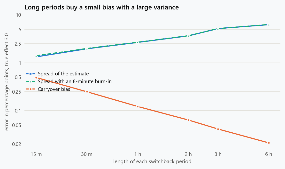
At fifteen-minute periods the burn-in throws away 53 percent of the orders and the estimator's spread rises by 3 percent, from 1.495 to 1.546. That is almost free, because the spread is set by the number of periods and the variation between them, not by the number of orders, and the burn-in does not change the number of periods. Meanwhile the bias disappears, the signal recovers its full size, and power rises from 39.8 to 50.2 percent. Discarding half the data made the test more sensitive.
The same table settles the period length question. Power falls steeply as periods lengthen: 50 percent at fifteen minutes with a burn-in, 32 at thirty, 20 at an hour, 11 at three hours. Shorter periods mean more independent draws of the market, and that is the only currency this design spends. The carryover bias that comes with them is handled by the burn-in rather than by lengthening the period, so the usual framing of a bias-variance tradeoff resolves in favour of short periods plus a burn-in.
Where the Design Still Fails
Two assumptions carry the whole argument. The first is that the carryover has a known, bounded length. If the effect persists for hours, as a change to driver incentives or to a recommendation model's training data might, no burn-in short enough to be affordable will remove it, and the switchback measures a blend of the two conditions. The test for this is to estimate the effect separately by position within the period and look for a gradient that has not flattened by the end.
The second is that assignment is balanced against the daily season. With six-hour periods, two weeks contains 56 draws, and it is entirely possible for treatment to land on more evening peaks than control. That imbalance is captured in the period-level standard error, which is why the coverage stays near 95 percent, but it makes the test weak. Blocking the randomisation, one treated and one control period within each pair of adjacent periods, removes most of it and is almost always worth doing.
What to Do
- Analyse at the unit you randomised. Period-level means with a standard error across periods; never an order-level or session-level standard error, which was wrong here by a factor of 15.
- Compute the design effect before the test to size it. One plus the orders per period times the within-period correlation tells you how many effective observations you have, and it is far fewer than the order count suggests.
- Choose the shortest period the system can switch cleanly, then add a burn-in at least as long as the carryover. Power comes from the number of periods, and the burn-in costs orders rather than periods.
- Measure the carryover length directly, by estimating the effect as a function of minutes since the switch, and set the burn-in from that rather than from a guess.
- Block the randomisation across adjacent periods or across the same hour on different days, so that the daily season cannot fall unevenly across arms.
- Check the estimate by position within the period after the test. A gradient that has not flattened means the burn-in was too short and the result is still attenuated.
The figure generator in the blog-reproducibility repository reproduces this article's figure; run it with --dry-run to print the numbers behind the figure without writing an image.
References
- Bojinov, I., Simchi-Levi, D., & Zhao, J. (2023). Design and analysis of switchback experiments. Management Science, 69(7), 3759-3777.
- Hu, Y., & Wager, S. (2022). Switchback experiments under geometric mixing. arXiv:2209.00197.
- Kish, L. (1965). Survey Sampling. Wiley.
- Donner, A., & Klar, N. (2000). Design and Analysis of Cluster Randomization Trials in Health Research. Arnold.
- Chamandy, N. (2016). Experimentation in a ridesharing marketplace. Lyft Engineering.
- Kohavi, R., Tang, D., & Xu, Y. (2020). Trustworthy Online Controlled Experiments: A Practical Guide to A/B Testing. Cambridge University Press.
Embed interactive plots, widgets, and demos using <figure>, <iframe>, or <div class="interactive-embed"> containers. Ensure each embed includes descriptive captions for accessibility.
How to cite
Use the quick export buttons to save citations for reference managers or copy the formatted text directly.
Diogo Ribeiro (2025). Switchback Experiments: Randomising Time When You Cannot Randomise Users. Faculty of Media Arts and Design, Technical University of Porto. https://diogoribeiro7.github.io/statistics/switchback_experiments_randomising_time/.

