Topics
Antibiotic resistance means that bacteria can withstand an antibiotic that would otherwise act against them. It does not mean that a person's body has become immune to the medicine. The CDC makes this distinction explicitly in its explanation of antimicrobial resistance. CDC overview.
The difference matters. If resistance were simply a personal habit formed by taking medicine, someone who had never used an antibiotic might seem protected from it. But resistant bacteria can spread between people, and bacteria can exchange resistance genes. A person's own prescription history is not the whole history of the microbes they encounter. CDC on how resistance spreads.
To understand one part of the process, we can begin with a population in which resistant bacteria are already present in small numbers.
Start with a rare minority
Imagine 100,000 bacteria of the same species in a hypothetical laboratory system. Of these, 99,900 belong to a group sensitive to a particular antibiotic, while 100 belong to a resistant group.
The resistant group is initially only 0.1% of the population.
Now impose a selective bottleneck: under the chosen conditions, suppose 1% of the sensitive group survives and 80% of the resistant group survives. These fractions are invented to make the arithmetic visible. They are not measurements for a named species, drug, concentration, or patient.
After this bottleneck, the model contains:
- 999 sensitive bacteria, down from 99,900;
- 80 resistant bacteria, down from 100.
Both groups have become smaller. Yet the resistant share has increased from 0.1% to about 7.4%, because the sensitive group fell much more sharply.
That is selection in the calculation. There is no need to assume that every surviving bacterium changed its identity or learned what the drug was trying to do.
Count bacteria and calculate their share separately
Repeat the same hypothetical bottleneck twice more, without adding growth or new bacteria between steps:
| Bottlenecks completed | Sensitive model count | Resistant model count | Resistant share of model counts |
|---|---|---|---|
| 0 | 99,900 | 100 | 0.1% |
| 1 | 999 | 80 | 7.4% |
| 2 | 9.99 | 64 | 86.5% |
| 3 | 0.0999 | 51.2 | 99.8% |
Fractional entries are expected counts in this mathematical illustration, not claims that a fraction of an individual bacterium exists. The displayed shares are ratios of those model counts. A real finite population would have integer counts and random variation, including the possibility that a small group disappears.
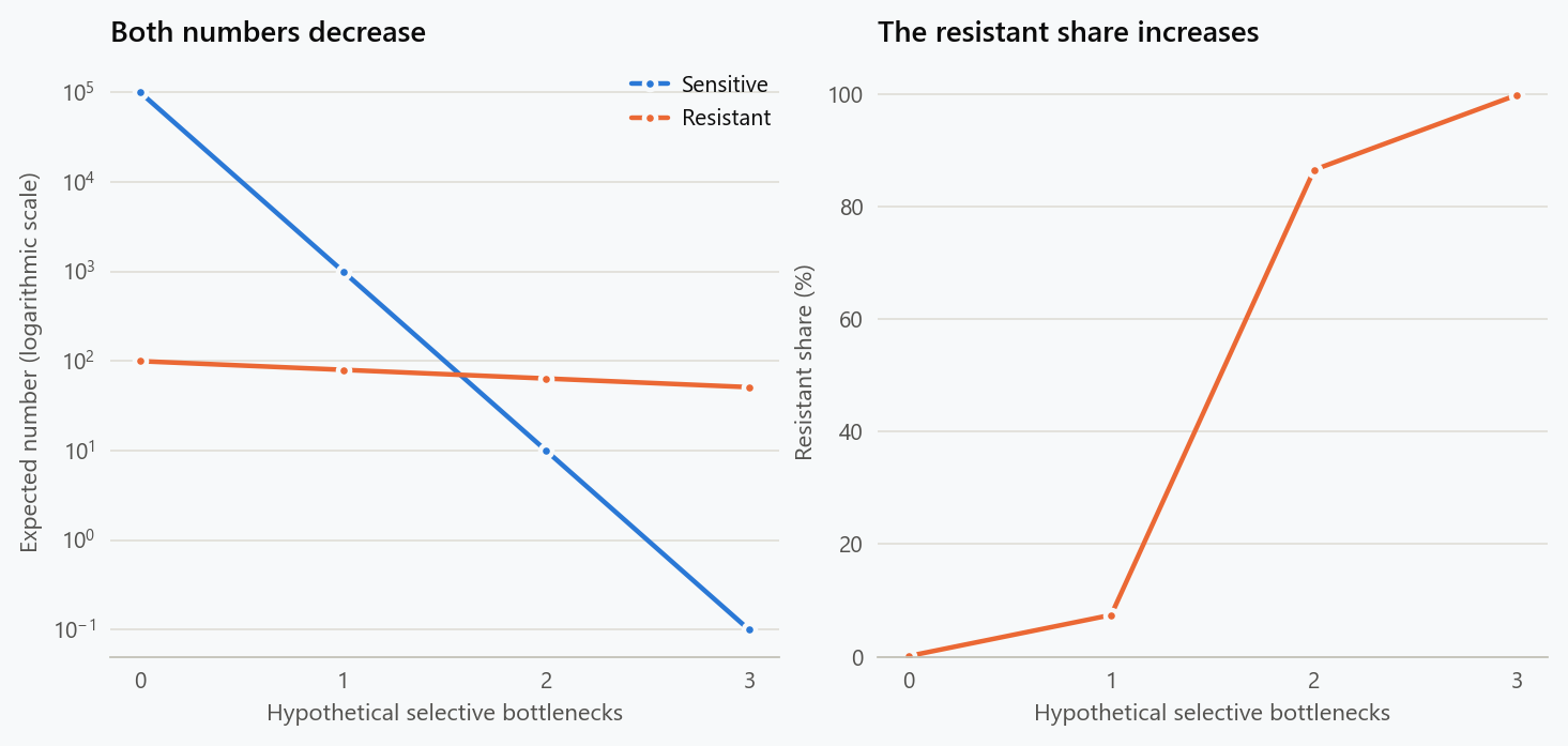
Original selection model. Sensitive and resistant survival fractions are fixed at 1% and 80%. There is no growth, mutation, transmission, or immune response. The horizontal axis does not represent prescribed doses.
The plots answer different questions. The first asks how many bacteria remain. The second asks which group makes up those survivors.
After the third step, resistance is almost universal in the model's remaining population, even though the resistant count itself has nearly halved. Saying only “resistance increased” would leave this distinction hidden.
Why the proportions change so quickly
The resistant group survives each bottleneck at 80 times the fraction of the sensitive group: $0.80/0.01=80$.
Before the first bottleneck, the ratio of resistant to sensitive counts is $100/99{,}900$. Afterwards it is $80/999$. The latter ratio is 80 times larger.
Each repeated bottleneck multiplies the resistant-to-sensitive ratio by the same factor. Starting from a very small fraction does not prevent a group from becoming dominant if the conditions repeatedly favour it strongly enough.
This is a statement about relative survival under the assumed conditions. It does not say that resistant bacteria grow faster in every environment, that all antibiotics select in the same way, or that every exposure produces these changes.
The model identifies a mechanism that can alter a population's composition. Establishing its strength in a real system requires measurements.
Write the change in frequency as a general rule
Let $f$ be the resistant fraction before a bottleneck, and let $w_R$ and $w_S$ be the resistant and sensitive survival fractions. The surviving resistant count is proportional to $fw_R$; the surviving sensitive count is proportional to $(1-f)w_S$. Dividing by their sum gives
This expression makes the comparison explicit. For an interior starting fraction, resistance increases in proportion when $w_R>w_S$, remains at the same proportion when the survival fractions are equal, and decreases when $w_R<w_S$.
The corresponding resistant-to-sensitive odds are even simpler:
The multiplier depends on the relative survival of the groups. If both survival fractions were 80%, the population would shrink but its composition would stay unchanged. If resistant survival were 90% and sensitive survival 100% in another hypothetical environment, the resistant fraction would fall slightly, from 0.1% to about 0.0900%.
Those examples do not assert a universal fitness cost of resistance. They demonstrate why the environmental conditions belong in the explanation. A label such as “resistant” does not specify every growth and survival comparison in every setting.
The rule also exposes an assumption about inheritance. We have treated group membership as stable across the step. If cells acquire or lose the relevant genetic capability, we need additional transitions between groups. Changing a survival fraction cannot represent every biological process at once.
Add regrowth and the count story changes
Our original table deliberately froze reproduction. After its first bottleneck, there were 999 sensitive and 80 resistant expected survivors, with resistance at about 7.4%.
Suppose both groups now multiply by 100 before any further selective event. The resulting counts are 99,900 sensitive and 8,000 resistant bacteria. The resistant fraction stays at 7.4%, because multiplying both counts by the same factor does not change their ratio. The total population, however, rises to 107,900, and the resistant count is now 80 times its original value of 100.
Equal regrowth therefore changes the absolute-count conclusion without changing the composition produced by selection. That is why observing a rising resistant fraction is insufficient to reconstruct the bacterial load.
Now try a different, explicitly hypothetical growth comparison. Multiply the 999 sensitive survivors by 100 but the 80 resistant survivors by 20:
| State | Sensitive count | Resistant count | Resistant fraction |
|---|---|---|---|
| After the first bottleneck | 999 | 80 | 7.41% |
| Both groups multiply by 100 | 99,900 | 8,000 | 7.41% |
| Sensitive multiply by 100; resistant by 20 | 99,900 | 1,600 | 1.58% |
The final two rows are alternative continuations from the first row, not successive stages. In the unequal-growth continuation, resistance becomes a smaller fraction than immediately after the bottleneck, while its count increases substantially. A falling proportion can coexist with more resistant bacteria.
These scenarios explain why the timing of measurements matters. A sample taken immediately after a selective event and one taken after regrowth can describe different population states. The growth multipliers are invented; using them to schedule or evaluate a treatment would require biological and clinical information that this example does not contain.
A rare group can disappear by chance
Expected counts smooth over the discreteness of individual bacteria. To see what that smoothing hides, suppose each initially resistant cell independently survives one bottleneck with probability 0.8. With $R$ resistant cells at the start, the number of survivors follows a binomial distribution.
The expected count is $0.8R$, but the probability that all resistant cells disappear is
| Resistant cells initially | Expected resistant survivors | Probability of none surviving |
|---|---|---|
| 1 | 0.8 | 20% |
| 2 | 1.6 | 4% |
| 5 | 4.0 | 0.032% |
For one initial cell, the expected value 0.8 averages two outcomes: zero survivors or one survivor. No individual experiment contains 0.8 of a cell. That distinction becomes especially consequential when the population is small.
Independent survival is another model assumption, not a biological guarantee. Shared local conditions can make outcomes dependent. New genetic changes, immigration, or transfer can also reintroduce a capability after one local group disappears. The table isolates one stochastic mechanism; it does not estimate the probability of clearing an infection.
It also clarifies why a ratio of expected counts is not generally the expected value of a random ratio. Our original frequency table reports the former. If we wanted the distribution of resistant fractions across tiny replicate populations, we would need to model both random counts and decide how to treat replicates with no survivors at all.
Real bacteria add more routes to the story
Selection acts on differences. Our example supplies those differences at the start and then holds them fixed.
Real bacterial populations can also acquire new genetic changes and share genetic material. The CDC describes mobile genetic elements as one way resistance can move between germs. Resistant organisms can then spread through routes involving people, animals, food, and the environment. CDC transmission explanation.
These processes answer different questions. Selection helps explain why a variant becomes more common under particular conditions. Genetic change and gene transfer help explain where a capability comes from. Transmission helps explain how organisms or their resistance mechanisms reach new settings.
Keeping those questions separate avoids two opposite errors: suggesting that antibiotics make every bacterium deliberately adapt, or suggesting that resistant bacteria must always have been present in exactly their current form.
Resistance is specific enough to require evidence
Calling bacteria “resistant” needs a reference: resistant to which antimicrobial, assessed under which conditions? A bacterium does not have to resist every medicine to create a serious treatment problem. CDC overview.
Likewise, an unsuccessful treatment is an observation requiring assessment, not a diagnosis of resistance on its own. The two-population table contains no symptoms, laboratory results, drug concentrations in tissue, or competing explanations for illness.
Its numbers therefore cannot tell someone which medicine to take or how long to take it. They also cannot tell a clinician whether a particular patient's infection has cleared. Treating each row as another dose would silently turn a teaching example into a clinical model that it was never designed to be.
A surveillance percentage depends on who was sampled
Population composition matters at another level: the collection of isolates sent for testing. Consider two fictional settings in which the measured resistant fractions remain unchanged. Setting A has 20% resistant isolates; setting B has 60%.
In one reporting period, a surveillance dataset contains 900 tested isolates from A and 100 from B. In another, it contains 100 from A and 900 from B. The expected pooled proportions are
The headline percentage more than doubles even though neither setting's rate changes. This invented example does not explain any particular surveillance report. It demonstrates why changes in the composition of a sample can alter an aggregate statistic.
A responsible comparison would report the contributing settings and their sample sizes, check whether inclusion and testing procedures changed, and examine the within-setting results. Reweighting both periods to the same mixture can answer a different, more comparable question. With equal weights for A and B, both periods give 40%.
None of this means that an observed increase should be dismissed. The pooled result could reflect a meaningful shift in the patients or settings represented, a biological change within settings, or both. The point is to identify which population the denominator represents before assigning a mechanism to the trend.
There is a chain of questions between a social-media statement and a biological conclusion: which organism and drug, which laboratory definition, which sampling frame, which time interval, and which outcome? A proportion among selected tested isolates is not automatically a population-wide infection rate, just as a resistant fraction in our laboratory model is not a total bacterial count.
What the distinction changes in a conversation
If someone says, “My body has become resistant to antibiotics,” a useful correction is:
Antibiotic resistance concerns bacteria and the medicines acting on them. Some bacteria may survive better than others, and resistant bacteria or resistance genes can spread. The explanation is about the microbes, not the body becoming accustomed to the drug.
This wording also avoids assigning the entire problem to one person's behaviour. A resistant infection can reflect transmission and a much wider history of selection. Understanding the mechanism makes infection prevention and careful antibiotic use parts of the same public-health problem.
The calculation offers another useful question for a graph or headline: did the number of resistant bacteria rise, did their proportion rise, or did both rise? Those descriptions can imply very different population changes.
Reproduce the model
1
2
3
4
5
6
7
8
sensitive, resistant = 99_900.0, 100.0

for bottleneck in range(4):
    share = resistant / (sensitive + resistant)
    print(f"{bottleneck}: sensitive={sensitive:g}, "
          f"resistant={resistant:g}, resistant share={share:.1%}")
    sensitive *= 0.01
    resistant *= 0.80
The regrowth, extinction, and surveillance examples can also be checked directly:
1
2
3
4
5
6
7
8
for growth_s, growth_r in [(100, 100), (100, 20)]:
    sensitive, resistant = 999 * growth_s, 80 * growth_r
    print(sensitive, resistant, f"resistant fraction={resistant / (sensitive + resistant):.2%}")
for initial in (1, 2, 5):
    print(initial, f"extinction probability={0.2**initial:.3%}")
for tested_a, tested_b in [(900, 100), (100, 900)]:
    pooled = (0.2 * tested_a + 0.6 * tested_b) / (tested_a + tested_b)
    print(tested_a, tested_b, f"pooled resistance={pooled:.0%}")
The figure generator reproduces the original two panels. The accompanying checks verify that the resistant share increases while both model counts decrease.
Archive note: dated 20 March 2025 for this collection; written and source-checked on 18 September 2026.
Embed interactive plots, widgets, and demos using <figure>, <iframe>, or <div class="interactive-embed"> containers. Ensure each embed includes descriptive captions for accessibility.
How to cite
Use the quick export buttons to save citations for reference managers or copy the formatted text directly.
Diogo Ribeiro (2025). How Antibiotic Resistance Spreads Through Bacteria. Faculty of Media Arts and Design, Technical University of Porto. https://diogoribeiro7.github.io/science-communication/how_antibiotic_resistance_spreads/.