Optional Stopping: What a Daily Check Costs, and Three Rules That Make It Legal

The experiment was scheduled for four weeks. On the morning of day five the dashboard showed a 5.4 percent lift with a p-value of 0.04, the feature shipped, and the quarterly review recorded a win. Nothing about that sequence involves misconduct. The test statistic really did clear the threshold, the arithmetic behind the p-value was correct, and the analyst stopped because the answer had arrived.

The problem is the rule, not the arithmetic. A p-value below 0.05 means that data this extreme arises in one experiment in twenty when the test is applied once. Applying it every morning and stopping at the first crossing is a different procedure, with a different error rate, and the difference is not small.

Twenty-Eight Chances to Be Unlucky

The simulation runs twenty-eight days of an experiment at 225 users per arm per day, with a continuous per-user outcome of standard deviation 10 on a baseline of 20. That is the shape of a revenue-per-user or minutes-per-user metric. Each experiment is evaluated after every day, using the cumulative data so far.

Alongside the simulation there is an exact calculation. The cumulative test statistic is a random walk, and the probability that it ever leaves a set of boundaries can be computed by carrying the density of the partial sum forward look by look and deleting the part that has already crossed. That recursion is due to Armitage, McPherson and Rowe, and it needs no simulation at all.

1
2
3
4
5
6
7
8
9
10
11
12
13
14
15
16
17
18
19
20
21
22
23
24
25
26
27
28
29
30
31
32
33
34
35
36
37
38
39
40
41
42
43
44
45
46
47
48
49
50
51
52
53
54
55
import numpy as np
from scipy import stats
from scipy.signal import fftconvolve

RNG = np.random.default_rng(7)

SIGMA = 10.0          # per-user standard deviation of the outcome
PER_DAY = 225         # users per arm per day
DAYS = 28
REPS = 20000
ZC = stats.norm.ppf(0.975)


def daily_z(reps, delta=0.0, per_day=PER_DAY, days=DAYS, sigma=SIGMA, rng=RNG):
    """The running estimate, its standard error and its z score after each day."""
    n = per_day * np.arange(1, days + 1)                    # users per arm so far
    inc = rng.normal(delta * per_day, sigma * np.sqrt(per_day), (reps, days))
    inc -= rng.normal(0.0, sigma * np.sqrt(per_day), (reps, days))
    diff = np.cumsum(inc, axis=1) / n
    se = sigma * np.sqrt(2.0 / n)
    return diff, se, diff / se


def look_days(k, days=DAYS):
    """k evenly spaced looks, the last one on the final day."""
    return np.unique(np.round(np.arange(1, k + 1) * days / k).astype(int)) - 1


def crossing_prob(bounds, step=0.01, pad=8.0):
    """Probability that a random walk of unit-variance increments ever leaves
    `bounds`, which are given in z units, look by look. Armitage's recursion:
    carry the density of the partial sum forward, deleting the part that has
    already crossed. The grid has to hold the widest boundary the walk can
    still reach, so it is sized from the number of looks."""
    finite = np.asarray([b for b in bounds if np.isfinite(b)])
    span = finite.max() * np.sqrt(len(bounds)) + pad
    x = np.arange(-span, span + step, step)
    kernel = np.exp(-x ** 2 / 2) / np.sqrt(2 * np.pi) * step
    f = kernel.copy()                                        # density after look 1
    total = 0.0
    for k, b in enumerate(bounds, start=1):
        inside = np.abs(x) < b * np.sqrt(k)                  # z units to sum units
        total += f[~inside].sum()
        f = f * inside
        if k < len(bounds):
            f = fftconvolve(f, kernel, mode="same")
    return total


d0, se0, z0 = daily_z(REPS)
for k in (1, 2, 3, 4, 7, 14, 28):
    cols = look_days(k)
    simulated = (np.abs(z0[:, cols]) >= ZC).any(axis=1).mean()
    exact = crossing_prob(np.full(len(cols), ZC))
    print(f"{k:2d} looks: simulated {simulated:6.1%}   numerical recursion {exact:6.1%}")

Two independent methods agree to within half a percentage point, the recursion carrying a small upward bias from its grid. A weekly review over four weeks costs 12.7 percent. A daily check costs 27 percent. More than one experiment in four ends with a false winner, on data where the two arms are identical by construction.

The cost does not grow without limit. Each extra look adds less than the one before, because the statistic at day 20 is highly correlated with the statistic at day 19, and correlated tests are nearly the same test. The recursion answers the question directly: hold the horizon at twenty-eight days, keep the first look at the end of day one, and monitor more and more often.

1
2
3
4
5
for name, sub, step in (("daily", 1, 0.01), ("every 6 hours", 4, 0.01),
                        ("hourly", 24, 0.02), ("every 10 minutes", 144, 0.05)):
    steps = 28 * sub
    bounds = np.where(np.arange(1, steps + 1) >= sub, ZC, np.inf)
    print(f"{name:18s} {steps:6d} looks: {crossing_prob(bounds, step=step):.1%}")

Watching a live dashboard as closely as anyone realistically can costs about 41 percent rather than 5. The curve flattens because a look ten minutes after the last one is almost the same test, not because the procedure becomes safe.

What the Winner Looks Like

The error rate is only half the damage. A test that stops at the first crossing stops precisely when the noise is at its most flattering, and it reports the estimate at that moment.

1
2
3
4
5
6
7
first = np.argmax(np.abs(z0) >= ZC, axis=1)
hit = (np.abs(z0) >= ZC).any(axis=1)
claimed = np.abs(d0[hit, :][np.arange(hit.sum()), first[hit]])
print(f"stopped at some point in 28 days: {hit.mean():.1%}")
print(f"mean effect it claimed: {claimed.mean():.3f}, "
      f"{claimed.mean() / 20 * 100:.1f}% of a 20-unit baseline, truth 0")
print(f"median day it stopped: {np.median(first[hit] + 1):.0f}")

The typical false winner is found on day five and credited with 5.5 percent. Early stops happen early because the standard error is still wide, so crossing requires a large apparent effect. The rule selects for exaggeration, and the exaggeration is what gets written into the quarterly review.

Spending a Budget Across Looks

None of this argues for never looking. It argues for deciding, in advance, how much of the 5 percent each look is allowed to spend. Two classical answers exist.

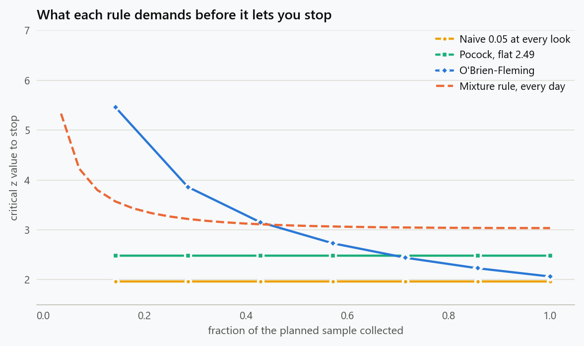
A Pocock boundary uses the same critical value at every look, chosen so that the whole sequence spends 5 percent. An O'Brien-Fleming boundary is severe early and lenient late, scaling as the inverse square root of accumulated information, so most of the budget is still unspent at the end. The recursion calibrates either shape directly.

1
2
3
4
5
6
7
8
9
10
11
12
13
14
15
16
17
18
19
20
21
22
def calibrate(shape, k=7, target=0.05):
    """Scale a boundary shape until the overall crossing probability is `target`."""
    lo, hi = 1.0, 8.0
    for _ in range(60):
        mid = (lo + hi) / 2
        if crossing_prob(mid * shape) > target:
            lo = mid
        else:
            hi = mid
    return (lo + hi) / 2 * shape


K = 7
pocock = calibrate(np.ones(K))
obf = calibrate(np.sqrt(K / np.arange(1, K + 1)))
for name, bound in (("Pocock", pocock), ("O'Brien-Fleming", obf)):
    print(f"{name:16s} " + " ".join(f"{b:5.2f}" for b in bound))
    print(f"{'  nominal alpha':16s} "
          + " ".join(f"{2 * (1 - stats.norm.cdf(b)):5.3f}" for b in bound))
    cols = look_days(K)
    mc = (np.abs(z0[:, cols]) >= bound).any(axis=1).mean()
    print(f"  crossing probability: recursion {crossing_prob(bound):.3%}, simulated {mc:.3%}")

Both spend the budget: the recursion puts Pocock at 5.000 percent and O'Brien-Fleming at 4.995 percent, and the simulation reads 4.91 and 4.98 percent. The two shapes express different attitudes. Pocock treats every look as equally worth stopping on and charges a flat 0.013 for the privilege. O'Brien-Fleming refuses to stop on the first week at anything short of a five-sigma result, and in exchange its final look is almost the unadjusted test, 2.06 against 1.96. A team that expects to run to the end unless something dramatic happens should prefer the second, because it barely taxes the final answer.

A Rule That Allows Unlimited Looks

Both boundaries assume the number of looks is fixed in advance. Dashboards are not like that: they are read whenever someone is curious. A rule that survives unlimited monitoring needs a different construction.

Take a normal prior of scale <div class="math-expression math-expression--source" data-math-alt="Mathematical expression" data-math-source="\tau" aria-label="Mathematical expression" tabindex="0">\(\tau\)</div> on the unknown effect and form the likelihood ratio of the data against the null, averaged over that prior. With <div class="math-expression math-expression--source" data-math-alt="_n" data-math-source="\hat\delta_n" aria-label="_n" tabindex="0">\(\hat\delta_n\)</div> the running estimate and <div class="math-expression math-expression--source" data-math-alt="V_n" data-math-source="V_n" aria-label="V_n" tabindex="0">\(V_n\)</div> its variance,

Under the null this quantity has expectation 1 at every <div class="math-expression math-expression--source" data-math-alt="n" data-math-source="n" aria-label="n" tabindex="0">\(n\)</div>, and it is a non-negative martingale. Ville's inequality then bounds the probability that it ever exceeds <div class="math-expression math-expression--source" data-math-alt="1/" data-math-source="1/\alpha" aria-label="1/" tabindex="0">\(1/\alpha\)</div> by <div class="math-expression math-expression--source" data-math-alt="Mathematical expression" data-math-source="\alpha" aria-label="Mathematical expression" tabindex="0">\(\alpha\)</div>, whatever stopping rule is used. So the test "reject when <div class="math-expression math-expression--source" data-math-alt="_n 20" data-math-source="\Lambda_n \ge 20" aria-label="_n 20" tabindex="0">\(\Lambda_n \ge 20\)</div>" holds its 5 percent under any amount of peeking, including looking continuously and stopping the instant it crosses.

1
2
3
4
5
6
7
8
9
10
11
12
13
14
15
16
17
18
19
20
21
22
23
24
25
26
27
28
def mixture_lr(diff, se, tau):
    """Mixture likelihood ratio against a normal prior of scale tau on the effect.
    Its running maximum bounds the error rate at any number of looks."""
    v = se ** 2
    return np.sqrt(v / (v + tau ** 2)) * np.exp(tau ** 2 * diff ** 2 / (2 * v * (v + tau ** 2)))


TAU = 0.5      # prior scale: a 2.5% change on a 20-unit baseline
for delta, label in ((0.0, "no effect"), (0.5, "2.5% effect")):
    diff, se, z = daily_z(REPS, delta=delta, rng=np.random.default_rng(23))
    cols = look_days(K)
    n_at = PER_DAY * (cols + 1)
    for name, bound in (("peek at 0.05, 7 looks", np.full(K, ZC)),
                        ("Pocock, 7 looks", pocock),
                        ("O'Brien-Fleming, 7 looks", obf)):
        crossed = np.abs(z[:, cols]) >= bound
        stop = crossed.any(axis=1)
        stop_n = np.where(stop, n_at[np.argmax(crossed, axis=1)], n_at[-1])
        print(f"{label:12s} {name:26s} stops {stop.mean():6.1%}   "
              f"mean users per arm {stop_n.mean():6.0f}")
    crossed = mixture_lr(diff, se, TAU) >= 1 / 0.05
    stop = crossed.any(axis=1)
    stop_n = np.where(stop, PER_DAY * (np.argmax(crossed, axis=1) + 1), PER_DAY * DAYS)
    print(f"{label:12s} {'mixture, all 28 days':26s} stops {stop.mean():6.1%}   "
          f"mean users per arm {stop_n.mean():6.0f}")
    print(f"{label:12s} {'fixed horizon, day 28':26s} "
          f"stops {(np.abs(z[:, -1]) >= ZC).mean():6.1%}   "
          f"mean users per arm {PER_DAY * DAYS:6d}")

The fixed-horizon test is the reference: 80.5 percent power at 6,300 users per arm, which is what the design was sized for. O'Brien-Fleming reaches 79.3 percent while using 4,923 users on average, a 22 percent saving for a power loss of one point. Pocock stops sooner still but pays nine points of power, because its flat boundary taxes the final look at 2.49 instead of 1.96 and some real effects that would have cleared 1.96 never clear 2.49.

The mixture rule is the conservative one. Its false positive rate under twenty-eight daily looks is 1.2 percent, well inside its 5 percent guarantee, and it detects the 2.5 percent effect only half the time. That is the price of a promise that holds for any stopping rule whatsoever, including ones chosen after seeing the data.

The Prior Scale Is a Real Choice

The mixture rule's efficiency depends on <div class="math-expression math-expression--source" data-math-alt="Mathematical expression" data-math-source="\tau" aria-label="Mathematical expression" tabindex="0">\(\tau\)</div>, the scale at which it expects effects to live. The guarantee holds for any <div class="math-expression math-expression--source" data-math-alt="Mathematical expression" data-math-source="\tau" aria-label="Mathematical expression" tabindex="0">\(\tau\)</div>; the speed does not.

1
2
3
4
5
6
7
8
9
for tau in (0.25, 0.5, 1.0, 2.0):
    for delta in (0.0, 0.5, 1.0):
        diff, se, _ = daily_z(REPS, delta=delta, rng=np.random.default_rng(41))
        crossed = mixture_lr(diff, se, tau) >= 1 / 0.05
        stop = crossed.any(axis=1)
        first_col = np.argmax(crossed, axis=1)
        n = np.where(stop, PER_DAY * (first_col + 1), PER_DAY * DAYS).mean()
        print(f"tau {tau / 20 * 100:4.1f}% of baseline, true effect {delta / 20 * 100:4.1f}%: "
              f"stops {stop.mean():6.1%}, mean users per arm {n:6.0f}")

Every row respects the 5 percent budget, so no choice of <div class="math-expression math-expression--source" data-math-alt="Mathematical expression" data-math-source="\tau" aria-label="Mathematical expression" tabindex="0">\(\tau\)</div> is invalid. But a scale far from the truth is slow: at 1.25 percent the rule detects a 2.5 percent effect 37.6 percent of the time, against 49.9 percent when the scale matches. Setting <div class="math-expression math-expression--source" data-math-alt="Mathematical expression" data-math-source="\tau" aria-label="Mathematical expression" tabindex="0">\(\tau\)</div> near the smallest effect worth shipping is the sensible default, and being wrong by a factor of two costs little.

Valid Does Not Mean Unbiased

There is one failure that no boundary fixes. Any rule that can stop early stops when the estimate is flattering, so the estimate at the stopping time overstates the effect. This is true even when the error rate is perfectly controlled.

1
2
3
4
5
6
7
8
9
10
11
12
13
14
15
16
17
18
19
diff, se, z = daily_z(REPS, delta=0.5, rng=np.random.default_rng(43))
cols = look_days(K)
rules = {
    "peek at 0.05, 7 looks": np.abs(z[:, cols]) >= ZC,
    "Pocock, 7 looks": np.abs(z[:, cols]) >= pocock,
    "O'Brien-Fleming, 7 looks": np.abs(z[:, cols]) >= obf,
}
for name, crossed in rules.items():
    stop = crossed.any(axis=1)
    at_stop = diff[:, cols][np.arange(REPS), np.argmax(crossed, axis=1)][stop]
    print(f"{name:26s} reports {at_stop.mean() / 20 * 100:5.2f}% "
          f"(truth 2.50%), exaggeration {at_stop.mean() / 0.5 - 1:+6.1%}")
crossed = mixture_lr(diff, se, TAU) >= 1 / 0.05
stop = crossed.any(axis=1)
at_stop = diff[np.arange(REPS), np.argmax(crossed, axis=1)][stop]
print(f"{'mixture, all 28 days':26s} reports {at_stop.mean() / 20 * 100:5.2f}% "
      f"(truth 2.50%), exaggeration {at_stop.mean() / 0.5 - 1:+6.1%}")
print(f"{'fixed horizon, day 28':26s} reports {diff[:, -1].mean() / 20 * 100:5.2f}% "
      f"(truth 2.50%), exaggeration {diff[:, -1].mean() / 0.5 - 1:+6.1%}")

The truth is 2.5 percent in every row. The fixed-horizon test recovers it. Every early-stopping rule overstates it, and the rules that stop soonest overstate it most: the mixture rule, which can stop on any of twenty-eight days, reports 4.02 percent. The sequential machinery buys a correct decision, not a correct number.

This matters for planning. A feature stopped early at an apparent 4 percent lift will be budgeted as a 4 percent lift, and the following quarter will look like a shortfall. The fix is to separate the two questions. Use the sequential rule to decide whether to stop, then estimate the effect from the remaining data, from a holdout that was never used in the stopping decision, or with an explicit correction for the selection.

Choosing Before the Test Starts

The choice is really about what the looks are for. If they exist to catch a disaster, an O'Brien-Fleming boundary is the right instrument: it is nearly free at the end, and it will stop a five-sigma regression in week one. If they exist because the team cannot stop watching, a mixture rule is honest about that and charges for it. If nobody will actually act before the planned end, a fixed horizon is both the most powerful and the only one that reports the effect correctly.

What does not work is the rule that has no name: look every day, stop on 0.05, and describe the result as significant. That procedure has a 27 percent error rate and a systematic upward bias, and both are properties of the rule rather than accidents of any particular test.

What to Do

1. Decide the number of looks and the boundary before the first user is assigned, and write both into the test document alongside the sample size.
2. Default to an O'Brien-Fleming boundary when looks exist as a safety valve. It costs about one point of power and leaves the final test near the unadjusted threshold.
3. Use a mixture sequential rule when monitoring is genuinely continuous, and set its scale near the smallest effect worth shipping. Expect roughly half the power of a fixed-horizon test against effects at that scale.
4. Never read a nominal 0.05 from a dashboard that updates. If the platform shows one, ask what its boundary is; if there is none, the number is not a 5 percent test.
5. Report the effect from data that did not drive the stopping decision. An early stop is evidence that something happened, not a measurement of how much.
6. Size the test for the effect you would act on, so that stopping early is an exception rather than the plan. A test with 80 percent power at the horizon has little to gain from aggressive early stopping.

References

• Armitage, P., McPherson, C. K., & Rowe, B. C. (1969). Repeated significance tests on accumulating data. Journal of the Royal Statistical Society: Series A, 132(2), 235-244.
• Pocock, S. J. (1977). Group sequential methods in the design and analysis of clinical trials. Biometrika, 64(2), 191-199.
• O'Brien, P. C., & Fleming, T. R. (1979). A multiple testing procedure for clinical trials. Biometrics, 35(3), 549-556.
• Lan, K. K. G., & DeMets, D. L. (1983). Discrete sequential boundaries for clinical trials. Biometrika, 70(3), 659-663.
• Jennison, C., & Turnbull, B. W. (2000). Group Sequential Methods with Applications to Clinical Trials. Chapman and Hall.
• Johari, R., Koomen, P., Pekelis, L., & Walsh, D. (2017). Peeking at A/B tests: why it matters, and what to do about it. Proceedings of the 23rd ACM SIGKDD International Conference on Knowledge Discovery and Data Mining, 1517-1525.
• Johari, R., Koomen, P., Pekelis, L., & Walsh, D. (2022). Always valid inference: continuous monitoring of A/B tests. Operations Research, 70(3).
• Howard, S. R., Ramdas, A., McAuliffe, J., & Sekhon, J. (2021). Time-uniform, nonparametric, nonasymptotic confidence sequences. Annals of Statistics, 49(2), 1055-1080.
• Kohavi, R., Tang, D., & Xu, Y. (2020). Trustworthy Online Controlled Experiments: A Practical Guide to A/B Testing. Cambridge University Press.