Topics
Scientific conclusions are often described as uncertain. That description is usually correct, but it is easy to draw the wrong inference from it.
One common move is to treat uncertainty as if it equalised competing explanations. If scientists cannot be completely certain, the reasoning goes, then several explanations must remain equally plausible. A related version says that because every model contains assumptions and every measurement contains error, no explanation can deserve substantially more confidence than another.
Neither conclusion follows.
Uncertainty describes what is not known exactly. Comparative evidence describes how well different explanations account for what has been observed. These are related questions, but they are not the same question.
Two hypotheses can both remain possible while one predicts the observed data much better than the other. A model can carry substantial parameter uncertainty while still outperforming a competitor across the relevant range. A scientific assessment can state that uncertainty remains while also concluding that one explanation is much better supported by multiple independent lines of evidence.
The mathematical structure is straightforward once the quantities are separated.
Competing explanations make different predictions
Suppose two hypotheses make different predictions about a repeated binary observation.
Under hypothesis $H_1$,
Under hypothesis $H_2$,
Now observe ten independent successes.
The probability of those data under $H_1$ is
Under $H_2$,
The likelihood ratio is
Numerically,
The data are therefore about 58 times as probable under $H_1$ as under $H_2$, given the stated models and independence assumptions.
Nothing in this calculation says that $H_1$ is certainly true.
It says that these data discriminate strongly between the two specified explanations.
Both statements can therefore be true at once:
and
There is no contradiction.
Richard Royall's likelihood framework makes this comparative idea explicit. For two simple statistical hypotheses, the likelihood ratio measures how much more strongly the observed data support one model than the other. Other inferential frameworks answer additional questions, but the elementary comparison already shows why uncertainty does not imply equal evidential support.
Equal prior plausibility is an additional assumption
Likelihood describes how well the observed data discriminate between specified models.
It does not by itself assign a probability that either model is true.
A Bayesian analysis adds prior information.
Let the prior probabilities of the two hypotheses be
and
Bayes' theorem can be written in odds form as
The first factor is the prior odds.
The second is the likelihood ratio or, for models with parameters integrated over prior distributions, the Bayes factor.
If the two hypotheses begin with equal prior probability, the prior odds are
After observing the ten successes, the posterior odds become approximately
The posterior probability of $H_1$ is then
There is still about 1.7% posterior probability assigned to $H_2$ within this deliberately restricted two-model world.
The uncertainty has not disappeared.
The explanations are nevertheless far from equally plausible.
Evidence and prior plausibility should not be confused
Now change the prior information.
Suppose $H_1$ begins with prior odds of
against $H_2$.
Instead of ten successes, suppose we observe nine successes and one failure.
The likelihood ratio is
The data favor $H_1$ over $H_2$ by almost ten to one.
The posterior odds are
This corresponds to posterior probability
So the data favor $H_1$, but $H_2$ remains more probable after the update because $H_1$ began with much lower prior plausibility.
That distinction is important.
The statement
is not identical to
The first is comparative evidence from the observed data under the stated models.
The second combines that evidence with information represented by the prior odds.
Arguments about scientific plausibility often become confused because these two quantities are mixed together.
Prior information is not permission to choose arbitrary beliefs
The existence of prior information does not make every prior equally defensible.
A prior can be informed by previous experiments, physical constraints, established mechanisms, prevalence, measurement characteristics, earlier datasets, or a formal hierarchical model.
It can also be chosen poorly.
If prior odds dominate the conclusion, their justification becomes part of the scientific argument.
Sensitivity analysis is useful here. Suppose several reasonable prior specifications all produce similar posterior conclusions. The result is less dependent on the subjective or conventional part of the analysis. If modest changes to the prior reverse the conclusion, that sensitivity should be reported rather than hidden.
The same principle applies outside explicitly Bayesian analysis. Background knowledge always constrains scientific interpretation. A proposed explanation that violates well-tested physical constraints does not begin on equal footing with one that is consistent with them merely because both can be stated verbally.
Scientific openness does not require assigning equal initial credibility to every imaginable explanation.
A likelihood ratio compares only the hypotheses that were included
The previous examples contain a deliberate simplification.
They assume that either $H_1$ or $H_2$ provides the relevant explanation.
Reality may contain another possibility, $H_3$.
Suppose the data strongly favor $H_1$ over $H_2$:
That does not establish that $H_1$ is a good model in absolute terms.
It establishes that $H_1$ fits the observed data better than $H_2$ according to the likelihood comparison.
A third model could satisfy
Or all three models could fit poorly in ways not captured by the particular statistic being examined.
Comparative support is therefore conditional on the model set.
This is one reason model checking and model comparison are distinct tasks.
A model can win a competition among weak alternatives.
Winning does not certify adequacy.
Uncertainty has several different sources
The word uncertainty is too broad to carry much scientific meaning unless its source is identified.
Suppose a quantity of interest is $\theta$. At least several kinds of uncertainty can affect inference about it.
Sampling uncertainty
Different random samples produce different estimates.
If
then the realised estimate varies around the underlying quantity even when the model is correct.
Increasing the effective sample size can often reduce this uncertainty.
Measurement uncertainty
The observed variable may differ from the quantity intended to be measured.
A generic measurement model is
Even a large sample does not recover $T$ accurately if systematic measurement error remains unaddressed.
Parameter uncertainty
A model structure may be accepted temporarily while some parameters remain poorly estimated.
Two parameter values can imply similar predictions over the observed domain.
Model uncertainty
Several functional forms or causal structures may remain compatible with the available evidence.
Parameter intervals calculated inside one model do not represent uncertainty about whether that model is the correct one.
Extrapolation uncertainty
A model may fit the observed domain well but behave differently from competitors outside that domain.
This uncertainty can increase sharply when prediction moves beyond the range where the model was tested.
Structural uncertainty
The set of relevant mechanisms, variables, or causal pathways may itself be incomplete.
This is especially important in complex systems where omitted processes can dominate under conditions not present in the original observations.
These uncertainties have different remedies.
Larger samples help with some.
Better instruments help with others.
New experiments, alternative models, or interventions may be needed for the rest.
Calling all of them simply "uncertainty" obscures what further evidence would actually resolve the problem.
Wide uncertainty does not imply a flat comparison
Suppose a parameter estimate is
with standard error
A conventional approximate 95% interval is
which gives
That is a broad range.
Now consider two hypotheses:
and
Under a normal sampling model,
The likelihood ratio favoring $H_A$ over $H_B$ is
This simplifies to
which is approximately
The parameter remains uncertain over a broad range.
The particular alternative $\theta=-10$ is nevertheless extremely poorly supported relative to $\theta=10$ under the stated model.
Uncertainty about magnitude is therefore not the same as uncertainty about sign, and uncertainty about sign is not the same as equal support for every possible value.
Confidence should reflect evidence and agreement, not theatrical certainty
Formal scientific assessments often need language that communicates uncertainty without creating the impression that every conclusion is equally tentative.
The IPCC provides one explicit example.
Its assessment framework distinguishes confidence from likelihood.
Confidence is based on characteristics such as the type, amount, quality, and consistency of evidence together with the degree of agreement across lines of evidence.
Likelihood is used when uncertainty can be expressed probabilistically.
This distinction is useful because a scientific conclusion can have several dimensions of support.
A probability estimate may be numerically precise but depend on a narrow model.
Another conclusion may resist precise probability assignment while being supported by many independent observations and strong mechanistic understanding.
Reducing both to a single binary label such as "certain" or "uncertain" destroys information.
The National Academies has made a similar point in its work on science communication. Uncertainty is intrinsic to many scientific questions, but communication should convey the weight of evidence rather than allowing uncertainty itself to erase differences in support.
Independent lines of evidence can create asymmetric plausibility
Suppose hypothesis $H_1$ predicts observations from three largely independent evidence streams, $D_1$, $D_2$, and $D_3$.
If conditional independence is a reasonable approximation, the likelihood ratio is
Assume the individual likelihood ratios are
The combined ratio is
No single piece of evidence is decisive.
Together they can create substantial discrimination.
This structure helps explain why scientific confidence can become strong gradually rather than through one dramatic experiment.
Replication, different measurement methods, mechanistic evidence, observational patterns, and intervention studies can all contribute distinct information.
Their value is greatest when their errors and assumptions are not all the same.
Ten analyses of the same biased dataset do not provide ten independent lines of evidence.
Independent convergence is stronger because it is harder for one failure mode to explain all of the observations simultaneously.
Agreement alone is not evidence
Multiple sources pointing in the same direction can still be misleading if they share the same underlying bias.
Suppose three instruments are calibrated against the same incorrect standard.
Their measurements may agree closely.
That agreement does not remove the common calibration error.
The same problem occurs in scientific literature. Several studies can use the same flawed measurement, the same selection mechanism, the same unrecognised confounder, or the same model assumption.
The number of agreeing studies is therefore not enough.
The structure of their dependence matters.
This is why independent methods are often more informative than repeated applications of the same method.
Scientific consensus is strongest when agreement survives variation in data, design, measurement, analytical approach, and research group.
Failure to reject an alternative is not evidence of equality
Another route to false equivalence begins with a negative result.
Suppose hypothesis $H_2$ has not been rejected by a statistical test.
It does not follow that
and
are equally supported.
A test can fail to reject because the sample is small, the measurement is noisy, the hypotheses make similar predictions over the observed region, or the statistic used has little power to distinguish them.
Absence of decisive evidence is not automatically evidence of equal plausibility.
The appropriate question is how much discrimination the study was capable of producing.
If two models make nearly identical predictions for the available experiment, the data may genuinely contain little comparative information.
If they make very different predictions and the observations consistently match one model, equal treatment is harder to justify.
A p-value does not rank explanations directly
P-values create another source of confusion.
A p-value is calculated under a null model. It is not generally the posterior probability that the null model is true, nor is it a direct likelihood ratio comparing two scientific explanations.
Berger and Sellke demonstrated in a point-null setting that conventional p-values can differ substantially from Bayesian measures of evidence against the null.
The broader lesson is not that every analysis should use a Bayes factor.
It is that inferential quantities answer different questions.
A p-value can be useful for evaluating how surprising a statistic would be under a null model.
A likelihood ratio compares how well two specified models predict the observed data.
A posterior probability combines evidence with prior information.
A confidence interval describes uncertainty under repeated-sampling assumptions.
Treating these outputs as interchangeable encourages precisely the kind of false certainty or false equivalence that careful scientific reasoning should avoid.
Model uncertainty can dominate parameter uncertainty
Suppose two models estimate the same quantity:
Within each model, the standard error is only 0.5.
If we report the estimate from $M_1$ as
the result looks extremely precise.
That interval says nothing about uncertainty caused by choosing $M_1$ rather than $M_2$.
A narrow interval conditional on one model can therefore coexist with substantial uncertainty across models.
Bayesian model averaging, multimodel inference, specification curves, robustness analysis, and related methods address this problem in different ways.
No single technique is universally appropriate.
The general principle is that uncertainty should be measured at the level where the scientific choice was made.
If model selection was uncertain, reporting only conditional parameter uncertainty understates the inferential problem.
Equal plausibility requires evidence, not politeness
Scientific communication sometimes adopts a conversational norm of giving competing explanations equal space.
That can be useful when several explanations genuinely have comparable support.
It becomes misleading when rhetorical balance is substituted for evidential balance.
If one hypothesis predicts the observations poorly, conflicts with established constraints, and lacks independent support, while another predicts several evidence streams successfully, describing them as "two equally possible explanations" is not neutrality.
It is an inaccurate description of the evidence.
The same principle applies in the opposite direction. Strong support does not justify caricaturing weaker alternatives or ignoring uncertainty that remains.
The scientifically appropriate goal is not equal treatment.
It is proportionate treatment.
The degree of confidence should track the quality and discriminatory power of the evidence.
Strong evidence can coexist with a nonzero chance of error
Suppose the posterior probability of an explanation is
There remains a probability of
assigned elsewhere within the model.
That residual uncertainty is real.
It does not follow that the 1% alternative deserves half of the discussion, half of the decision weight, or half of the scientific credibility.
Similarly, an engineering component designed to fail with probability (10^{-6}) is not certain to survive.
The nonzero failure probability does not make survival and failure equally likely.
Probability is explicitly designed to represent unequal uncertainty.
The phrase "we cannot be completely certain" therefore contains very little comparative information on its own.
We need to know what possibilities remain, how much probability or evidential support they receive, and why.
Decision uncertainty is not the same as scientific uncertainty
Even when one explanation is much more plausible, a decision can remain difficult.
Suppose the probability of a harmful event is estimated as
under action $A$ and
under action $B$.
The evidence may strongly support the ordering.
Whether the difference justifies choosing $A$ depends on costs, benefits, reversibility, alternatives, and consequences of error.
Decision theory therefore adds quantities beyond evidential plausibility.
Conversely, a decision can be easy even when scientific uncertainty is substantial.
If one action is cheap and reversible while another carries severe downside risk, the preferred action may be clear without precise knowledge of every parameter.
Scientific inference and decision making are connected.
They are not identical problems.
Some uncertainty is irreducible under the available design
Not every uncertainty can be eliminated by collecting more observations of the same type.
Suppose two causal models produce exactly the same observational distribution.
Then no amount of additional passive observation from that same distribution can distinguish them.
An intervention, a new measurement, or an external assumption may be required.
Similarly, structurally nonidentifiable parameters cannot be separated merely by repeating an experiment that only identifies their product.
This matters because vague calls for "more research" can be scientifically empty.
The useful question is what observation would cause the competing explanations to make different predictions.
Evidence becomes discriminating when the experiment reaches a part of the system where the models disagree.
Good uncertainty statements identify what could change the conclusion
A scientifically useful uncertainty statement should do more than say that the result is provisional.
It should indicate the source of the uncertainty and, where possible, the evidence that would reduce it.
For example:
- Sampling uncertainty could be reduced by a larger independent sample.
- Measurement uncertainty could require a better instrument or validation study.
- Model uncertainty could require testing alternative functional forms.
- Causal ambiguity could require intervention or a valid natural experiment.
- Extrapolation uncertainty could require observations in the target domain.
- Mechanistic uncertainty could require direct measurement of the proposed pathway.
This language is more informative than presenting uncertainty as a single cloud surrounding the conclusion.
It also makes scientific disagreement easier to interpret.
Researchers can agree about the data and disagree about which uncertainty matters most.
That is different from having no evidence at all.
The question is not whether doubt exists
Return to the first example.
Ten successes are observed.
Under $H_1$,
Under $H_2$,
The likelihood ratio is approximately
There is still uncertainty. A model with success probability 0.6 can produce ten successes. The probability is small but not zero.
What the data do not support is the statement that the two explanations are equally plausible merely because neither can be ruled out with logical certainty.
Scientific inference rarely works by eliminating every logically possible alternative.
It works by comparing how well explanations survive contact with evidence, by testing predictions that discriminate among them, and by updating confidence as independent evidence accumulates.
That process can leave room for error while producing very unequal support.
Uncertainty is therefore not the opposite of knowledge.
It is part of the description of how strong the knowledge is.
The important scientific question is not whether uncertainty remains.
It is how much remains, where it enters, and whether the competing explanations deserve the same weight in light of the evidence.
Often they do not.
References
Berger, J. O., & Sellke, T. (1987). Testing a point null hypothesis: The irreconcilability of P values and evidence. Journal of the American Statistical Association, 82(397), 112–122. https://doi.org/10.1080/01621459.1987.10478397
Intergovernmental Panel on Climate Change. (2021). Framing, context and methods. In Climate Change 2021: The Physical Science Basis. Cambridge University Press.
Kass, R. E., & Raftery, A. E. (1995). Bayes factors. Journal of the American Statistical Association, 90(430), 773–795. https://doi.org/10.1080/01621459.1995.10476572
National Academies of Sciences, Engineering, and Medicine. (2017). Communicating Science Effectively: A Research Agenda. Washington, DC: The National Academies Press. https://doi.org/10.17226/23674
Royall, R. M. (1992). The elusive concept of statistical evidence. In J. M. Bernardo, J. O. Berger, A. P. Dawid, & A. F. M. Smith (Eds.), Bayesian Statistics 4 (pp. 405–418). Oxford University Press.
Royall, R. M. (1997). Statistical Evidence: A Likelihood Paradigm. Chapman & Hall.
Royall, R. M. (2000). On the probability of observing misleading statistical evidence. Journal of the American Statistical Association, 95(451), 760–768. https://doi.org/10.1080/01621459.2000.10474264
Embed interactive plots, widgets, and demos using <figure>, <iframe>, or <div class="interactive-embed"> containers. Ensure each embed includes descriptive captions for accessibility.
How to cite
Use the quick export buttons to save citations for reference managers or copy the formatted text directly.
Diogo Ribeiro (2025). Scientific Uncertainty Does Not Make Every Explanation Equally Plausible. Faculty of Media Arts and Design, Technical University of Porto. https://diogoribeiro7.github.io/science-communication/scientific_uncertainty_does_not_make_every_explanation_equally_plausible/.