Topics
The analysis compared users who adopted a new feature against users who did not, adjusted for everything in the warehouse, and reported that adopters score 0.96 higher. The true effect is 0.30. Nothing in the output says so: the residuals behave, the covariates balance on what was measured, and the interval is narrow.
There is a way to see the problem anyway. Run the same comparison on an outcome the feature cannot possibly affect. If adopters also look better on that, the comparison is measuring who adopts rather than what adoption does. Here it reports 0.49 on an outcome with no causal path from the feature at all.
An Outcome the Treatment Cannot Touch
The simulation gives users an unobserved level of engagement that drives both adoption and the outcomes. The feature raises the real outcome by 0.30 and has no path at all to the negative control.
1
2
3
4
5
6
7
8
9
10
11
12
13
14
15
16
17
18
19
20
21
22
23
24
25
26
27
28
29
30
31
32
33
34
import numpy as np
from scipy import stats

RNG = np.random.default_rng(67)
N = 40000


def population(n, effect=0.30, conf_y=0.80, conf_n=0.60, conf_adopt=1.0, rng=RNG):
    """Users adopt a feature partly because of an unobserved level of
    engagement, which also drives both outcomes. The treatment moves the real
    outcome and cannot touch the negative control."""
    u = rng.normal(0, 1, n)                                  # unobserved engagement
    adopt = rng.random(n) < 1 / (1 + np.exp(-(conf_adopt * u - 0.5)))
    y = 5 + conf_y * u + effect * adopt + rng.normal(0, 1, n)
    # The negative control outcome shares the confounding and nothing else.
    ncontrol = 5 + conf_n * u + rng.normal(0, 1, n)
    return adopt, y, ncontrol, u


def naive(adopt, outcome):
    a, b = outcome[~adopt], outcome[adopt]
    d = b.mean() - a.mean()
    se = np.sqrt(a.var(ddof=1) / a.size + b.var(ddof=1) / b.size)
    return d, se


adopt, y, nc, u = population(N)
d_y, se_y = naive(adopt, y)
d_n, se_n = naive(adopt, nc)
print(f"adopters: {adopt.mean():.1%} of users")
print(f"apparent effect on the real outcome:     {d_y:+.3f} +- {se_y:.3f} (truth +0.300)")
print(f"apparent effect on the negative control: {d_n:+.3f} +- {se_n:.3f} (truth  0.000)")
print(f"bias visible in the negative control: {d_n:+.3f}, "
      f"actual bias in the real outcome: {d_y - 0.30:+.3f}")
| Quantity | Value |
|---|---|
| Share of users who adopt | 39.8% |
| Apparent effect on the real outcome | +0.960 ± 0.013 |
| True effect | +0.300 |
| Apparent effect on the negative control | +0.487 ± 0.012 |
| True effect on the negative control | 0 |
The negative control is unambiguous: an effect of 0.487 with a standard error of 0.012 on an outcome that cannot move. No amount of adjustment for measured covariates would have revealed that, because the problem is a variable nobody has.
Good negative control outcomes share the confounding and exclude the causal path. In product work they are usually metrics the feature has no route to: a user's behaviour in an unrelated surface, an outcome recorded before the feature existed, or an outcome the feature's mechanism cannot reach. In epidemiology the classic form is an outcome with the same selection into treatment and no biological link.
Does the Control Measure the Bias, or Just Announce It?
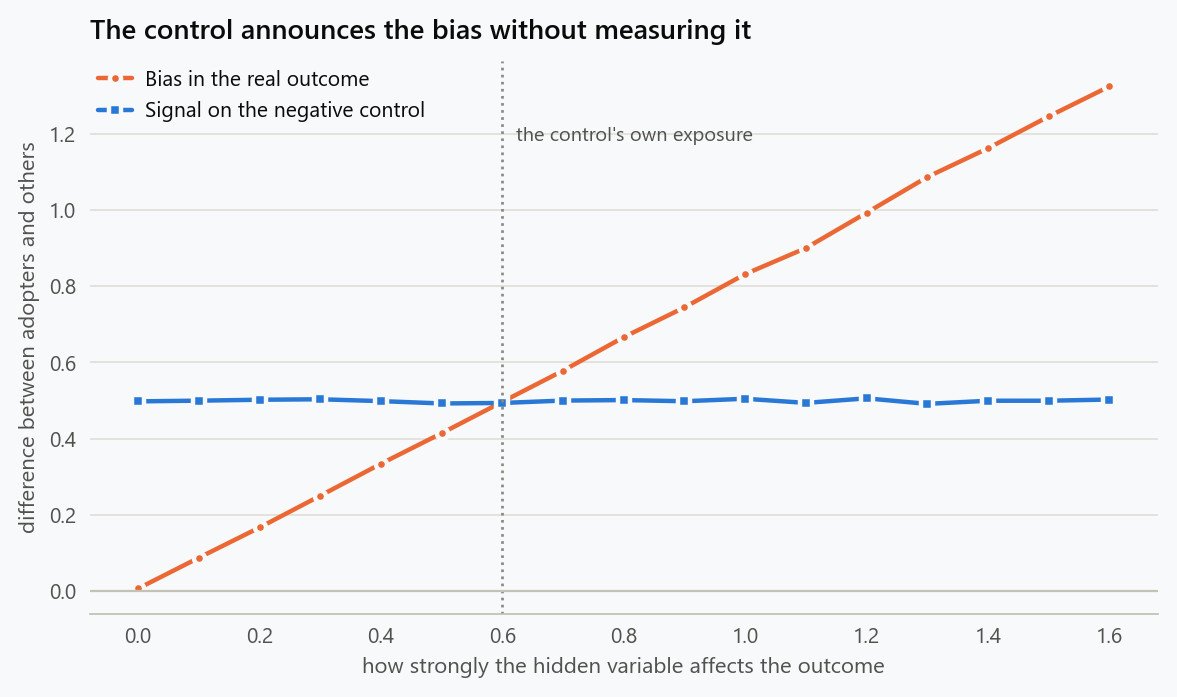
Detection is one thing. Teams usually want more, and try to read the control's signal as the size of the bias in the real outcome. That works only under a condition worth stating explicitly.
1
2
3
4
5
6
7
8
9
10
11
12
13
rows = []
for conf_y, conf_n in ((0.8, 0.6), (0.8, 0.8), (0.4, 0.6), (1.2, 0.6), (0.0, 0.6)):
    r = np.random.default_rng(3)
    by, bn = [], []
    for _ in range(60):
        adopt, y, nc, _ = population(20000, conf_y=conf_y, conf_n=conf_n, rng=r)
        by.append(naive(adopt, y)[0] - 0.30)
        bn.append(naive(adopt, nc)[0])
    rows.append((conf_y, conf_n, np.mean(by), np.mean(bn)))
    print(f"confounding on outcome {conf_y:4.1f}, on control {conf_n:4.1f}: "
          f"bias in the outcome {np.mean(by):+.3f}, "
          f"signal in the control {np.mean(bn):+.3f}, "
          f"ratio {np.mean(by) / np.mean(bn) if abs(np.mean(bn)) > 1e-9 else float('nan'):5.2f}")
| Confounding on the outcome | On the control | Bias in the outcome | Signal in the control | Ratio |
|---|---|---|---|---|
| 0.8 | 0.6 | +0.665 | +0.497 | 1.34 |
| 0.8 | 0.8 | +0.665 | +0.663 | 1.00 |
| 0.4 | 0.6 | +0.332 | +0.497 | 0.67 |
| 1.2 | 0.6 | +0.998 | +0.497 | 2.01 |
| 0.0 | 0.6 | −0.001 | +0.497 | 0.00 |
The ratio is the ratio of the two confounding strengths, up to sampling noise, which is the whole story in one column. When the control is affected by the hidden variable to the same degree as the outcome, its signal is the bias. When it is affected half as much, it understates the bias by half. And the last row is the case that costs credibility: the control screams while the real outcome is unbiased, because the hidden variable happens to touch one and not the other.
So a negative control is a strong detector and a weak estimator. A signal means the design cannot be trusted. The absence of a signal is weaker evidence than it feels, and the size of a signal is not the size of the bias unless there is an argument that the confounding acts equally on both.
How Much Bias It Can Catch
A control with weak exposure to the confounder needs data to show anything.
1
2
3
4
5
6
7
8
9
10
for n in (1000, 5000, 20000, 100000):
    r = np.random.default_rng(5)
    hits, sizes = 0, []
    for _ in range(400):
        adopt, y, nc, _ = population(n, conf_n=0.25, rng=r)
        d, se = naive(adopt, nc)
        hits += abs(d) > 1.96 * se
        sizes.append(d)
    print(f"{n:7,} users: control signal {np.mean(sizes):+.3f}, "
          f"flagged as non-zero {hits / 400:5.1%} of the time")
| Users | Signal on the control | Flagged as non-zero |
|---|---|---|
| 1,000 | +0.211 | 89.8% |
| 5,000 | +0.206 | 100.0% |
| 20,000 | +0.206 | 100.0% |
| 100,000 | +0.207 | 100.0% |
With a control only a quarter as exposed to the hidden variable as the outcome, a thousand users already catch it nine times in ten. That is the practical argument for running these checks routinely: they are cheap, and they work at sample sizes far below what the main analysis needs.
Correcting With the Control
The tempting next step is to subtract the control's signal from the estimate. It moves in the right direction and rarely arrives.
1
2
3
4
5
6
7
8
9
10
11
for conf_n in (0.6, 0.3, 0.9):
    r = np.random.default_rng(7)
    raw, corrected = [], []
    for _ in range(200):
        adopt, y, nc, _ = population(20000, conf_n=conf_n, rng=r)
        d_y = naive(adopt, y)[0]
        d_n = naive(adopt, nc)[0]
        raw.append(d_y)
        corrected.append(d_y - d_n)
    print(f"control carries {conf_n / 0.8:4.0%} of the outcome's confounding: "
          f"raw {np.mean(raw):+.3f}, corrected {np.mean(corrected):+.3f}, truth +0.300")
| Confounding the control carries, relative to the outcome | Raw estimate | Corrected | Truth |
|---|---|---|---|
| 75% | +0.964 | +0.466 | +0.300 |
| 37% | +0.964 | +0.715 | +0.300 |
| 112% | +0.964 | +0.217 | +0.300 |
Each correction removes most of the error and leaves a residue whose sign depends on whether the control is more or less exposed than the outcome, which is precisely the thing nobody can measure. Calibration by negative control is a defensible way to narrow a claim from "adopters score a point higher" to "somewhere between a fifth and a half of a point, and the design cannot do better than that". It is not a way to recover the causal effect.
The Experiment Version
Randomised experiments have their own negative control, and most teams already run it without using the name. An A/A test splits traffic between two identical experiences: any difference is instrumentation, assignment or logging, never the product.
1
2
3
4
5
6
7
8
9
10
11
for n_per_arm in (2000, 10000, 50000):
    for bias in (0.0, 0.02, 0.05):
        r = np.random.default_rng(11)
        hits = 0
        for _ in range(2000):
            a = r.normal(5, 1, n_per_arm)
            b = r.normal(5 + bias, 1, n_per_arm)      # an instrumentation difference
            se = np.sqrt(a.var(ddof=1) / n_per_arm + b.var(ddof=1) / n_per_arm)
            hits += abs(b.mean() - a.mean()) > 1.96 * se
        print(f"{n_per_arm:6,} per arm, hidden bias {bias:4.2f}: "
              f"A/A test flags it {hits / 2000:5.1%} of the time")
| Users per arm | No hidden bias | Bias of 0.02 | Bias of 0.05 |
|---|---|---|---|
| 2,000 | 5.2% | 10.3% | 35.5% |
| 10,000 | 4.4% | 29.3% | 94.8% |
| 50,000 | 5.9% | 88.9% | 100.0% |
The first column is the reassuring one: with no hidden bias the test flags a problem about five percent of the time, exactly as promised, which means a single A/A failure is not evidence of anything. The other columns set expectations. A small instrumentation bias of 0.02 on an outcome with unit spread is missed seven times in ten at ten thousand users per arm. An A/A test that passes at that size has ruled out gross problems and nothing subtle.
That is why A/A checks belong in the platform rather than in the test plan: run continuously across many pairs, their failures accumulate into a usable signal, while a single run before a launch mostly measures nothing.
What Makes a Good Control
The requirements are easy to state and take work to satisfy. It must share the selection, so whatever drives people into treatment must also drive their value on the control. It must exclude the causal path, so there must be a reason the treatment cannot reach it. And it must be measured with enough precision to detect a bias worth worrying about.
The most reliable source is time. An outcome recorded before the treatment existed cannot have been caused by it, shares whatever selection is at work, and is usually available in the same tables. Pre-period outcomes are the negative control that requires no argument.
What to Do
- Choose a negative control before running the analysis, and write down why the treatment cannot affect it. A control chosen afterwards is a result chosen afterwards.
- Prefer a pre-treatment measurement of the same outcome. It shares the selection by construction and needs no causal argument.
- Report the control's estimate and interval next to the main result every time, whether or not it is clean.
- Treat a signal as disqualifying for a causal claim, and treat a clean control as weak support rather than a licence.
- Do not subtract the control unless you can argue the confounding acts equally on both. Use it to bound the claim instead.
- Run A/A comparisons continuously in the experiment platform rather than once before launch, and size them against the smallest bias that would change a decision.
The figure generator in the blog-reproducibility repository reproduces this article's figure; run it with --dry-run to print the numbers behind the figure without writing an image.
References
- Lipsitch, M., Tchetgen Tchetgen, E., & Cohen, T. (2010). Negative controls: a tool for detecting confounding and bias in observational studies. Epidemiology, 21(3), 383-388.
- Shi, X., Miao, W., & Tchetgen Tchetgen, E. (2020). A selective review of negative control methods in epidemiology. Current Epidemiology Reports, 7(4), 190-202.
- Arnold, B. F., Ercumen, A., Benjamin-Chung, J., & Colford, J. M. (2016). Brief report: negative controls to detect selection bias and measurement bias in epidemiologic studies. Epidemiology, 27(5), 637-641.
- Schuemie, M. J., Ryan, P. B., DuMouchel, W., Suchard, M. A., & Madigan, D. (2014). Interpreting observational studies: why empirical calibration is needed to correct p-values. Statistics in Medicine, 33(2), 209-218.
- Rosenbaum, P. R. (2002). Observational Studies (2nd ed.). Springer.
- Kohavi, R., Tang, D., & Xu, Y. (2020). Trustworthy Online Controlled Experiments: A Practical Guide to A/B Testing. Cambridge University Press.
Embed interactive plots, widgets, and demos using <figure>, <iframe>, or <div class="interactive-embed"> containers. Ensure each embed includes descriptive captions for accessibility.
How to cite
Use the quick export buttons to save citations for reference managers or copy the formatted text directly.
Diogo Ribeiro (2026). Negative Controls: Measuring an Effect That Cannot Exist. Faculty of Media Arts and Design, Technical University of Porto. https://diogoribeiro7.github.io/statistics/negative_controls_finding_bias_you_cannot_see/.