Topics
An engineer regresses failure rate on operating temperature and finds an effect half the size the physics predicts. A data scientist trains a model on measurements from a calibrated laboratory rig and watches its error triple when it is deployed on the plant's own sensors. Both have met the same fact: noise in a predictor does something that noise in the outcome never does. It biases the answer, in a direction and by an amount that can be worked out.
Noise in the Outcome and Noise in the Predictor
Noise in the outcome is harmless in the sense that matters. If $y$ is measured with error, the fitted slope is unbiased and merely less precise. Noise in a predictor is different. Suppose the true relationship is $y = \beta x^* + e$ but what is recorded is $x = x^* + u$, with $u$ independent noise. Regressing $y$ on $x$ gives, in expectation,
The factor $\lambda$ is the reliability of the measurement: the share of its variance that is signal. A predictor whose variance is 60 percent signal and 40 percent noise has its slope shrunk to 60 percent of the truth, however large the sample. The bias does not average out, because the noise does not merely blur the relationship. It dilutes it, by spreading the same range of $y$ across a wider range of recorded $x$.
1
2
3
4
5
6
7
8
9
10
11
12
13
14
15
import numpy as np
from scipy.optimize import curve_fit
from sklearn.ensemble import RandomForestRegressor

rng = np.random.default_rng(0)
n = 20000

x_true = rng.normal(size=n)
y = 1.0 * x_true + rng.normal(scale=1.0, size=n)      # true slope 1
print("reliability   observed slope   theory")
for rel in (1.0, 0.8, 0.6, 0.4, 0.2):
    su = np.sqrt((1 - rel) / rel)                      # noise sd that gives this reliability
    x_obs = x_true + rng.normal(scale=su, size=n)
    slope = np.polyfit(x_obs, y, 1)[0]
    print(f"{rel:<13}{slope:>10.3f}        {rel:.3f}")
| Reliability of the predictor | Fitted slope | Predicted by $\beta\lambda$ |
|---|---|---|
| 1.0 | 1.003 | 1.000 |
| 0.8 | 0.808 | 0.800 |
| 0.6 | 0.601 | 0.600 |
| 0.4 | 0.397 | 0.400 |
| 0.2 | 0.196 | 0.200 |
Twenty thousand observations, and the slope is wrong by exactly the reliability. The same arithmetic applies to correlations, where Spearman derived it in 1904: the observed correlation is the true one times the square root of the product of the two reliabilities. A correlation of 0.5 between two quantities each measured with reliability 0.6 will be observed as 0.3.
The Bias Leaks Into Other Coefficients
With one predictor the damage is confined to that predictor's coefficient. With several, it spreads. A predictor that is measured with noise loses part of its coefficient, and any correlated predictor that is measured cleanly picks it up.
1
2
3
4
5
6
7
8
9
10
11
12
13
14
15
z = rng.normal(size=n)
x1 = z + rng.normal(scale=0.7, size=n)
x2 = z + rng.normal(scale=0.7, size=n)             # correlated with x1, no effect of its own
y2 = 1.0 * x1 + 0.0 * x2 + rng.normal(size=n)

def ols(X, y):
    X = np.column_stack([np.ones(len(X)), X])
    return np.linalg.lstsq(X, y, rcond=None)[0][1:]

print(f"corr(x1, x2) = {np.corrcoef(x1, x2)[0, 1]:.2f}")
print("noise sd on x1   coef x1   coef x2   (truth 1.0, 0.0)")
for su in (0.0, 0.5, 1.0, 1.5):
    x1_obs = x1 + rng.normal(scale=su, size=n)
    b = ols(np.column_stack([x1_obs, x2]), y2)
    print(f"{su:<16}{b[0]:>8.3f}{b[1]:>10.3f}")
| Noise added to $x_1$ (sd) | Coefficient of $x_1$ | Coefficient of $x_2$ |
|---|---|---|
| 0.0 | 0.999 | 0.000 |
| 0.5 | 0.761 | 0.159 |
| 1.0 | 0.447 | 0.369 |
| 1.5 | 0.263 | 0.496 |
The two predictors are correlated at 0.67, and only the first has any effect. As noise is added to it, its coefficient falls from 1.0 to 0.26 and the coefficient of the second, which does nothing, rises from zero to 0.50. The regression is not confused. Given noisy $x_1$, the clean $x_2$ genuinely carries information about $x_1^*$, and the fit uses it. But a reader of the coefficient table will conclude that both variables matter and that they matter about equally, and a reader of a feature importance chart will conclude the same.
The practical consequence is that comparisons between predictors are biased toward the better-measured one. A cheap, precise proxy will outrank the true cause it proxies for, if the cause is measured with noise. "Which variable matters most" cannot be answered from a fit alone when the variables differ in measurement quality, and in industrial data they almost always do.
Recovering the Slope
When the reliability is known, the correction is division. Repeated measurements of the same units, or a validation subsample measured with a reference instrument, give an estimate of $\operatorname{Var}(u)$, and the fitted slope divided by $\lambda$ is unbiased. This is regression calibration, and for a single linear predictor it is exact.
When the noise variance is known but the model is not linear, or the correction has to be applied to a fitted model rather than to a coefficient, simulation-extrapolation is the general tool. Add further noise to the predictor in known multiples of the existing noise, refit at each level, watch how the estimate degrades, and extrapolate the trend back to the level that would correspond to no noise at all.
1
2
3
4
5
6
7
8
9
10
11
12
13
14
15
16
17
18
rel = 0.6
su = np.sqrt((1 - rel) / rel)
x_obs = x_true + rng.normal(scale=su, size=n)
lams = np.array([0.0, 0.5, 1.0, 1.5, 2.0])            # added noise variance, as multiples
slopes = []
for lam in lams:
    s = [np.polyfit(x_obs + rng.normal(scale=np.sqrt(lam) * su, size=n), y, 1)[0]
         for _ in range(20)]
    slopes.append(np.mean(s))
slopes = np.array(slopes)

quadratic = np.polyval(np.polyfit(lams, slopes, 2), -1.0)
rational = lambda lam, a, b: a / (b + lam)
(a, b), _ = curve_fit(rational, lams, slopes, p0=[1.0, 2.0])
print(f"slopes at added-noise multiples {lams.tolist()}: {slopes.round(3).tolist()}")
print(f"quadratic extrapolant at -1: {quadratic:.3f}; rational extrapolant at -1: "
      f"{rational(-1.0, a, b):.3f}; regression calibration: {slopes[0] / rel:.3f}; truth 1.0")
print(f"fitted denominator b = {b:.2f}; theory (var(x*) + var(u)) / var(u) = {(1 + su**2) / su**2:.2f}")
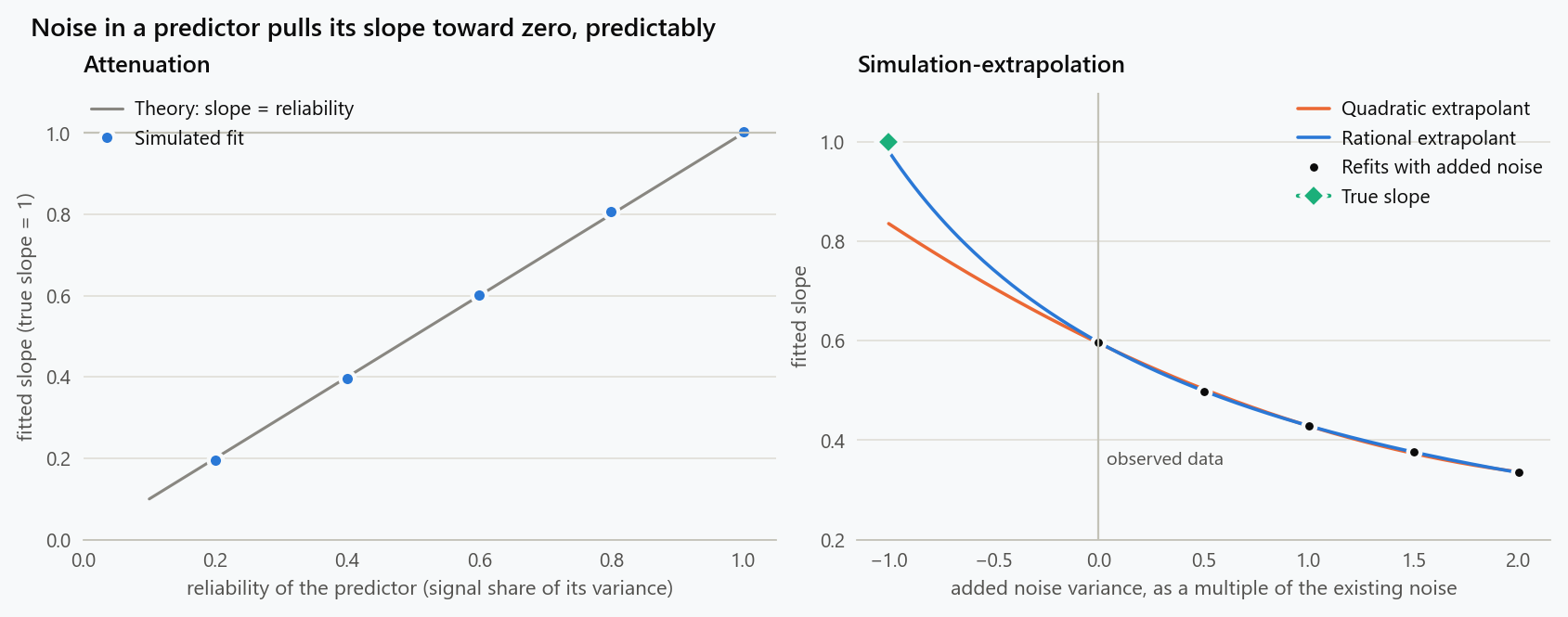
With reliability 0.6 the naive slope is 0.597. Adding noise at half, once, one and a half times and twice the existing variance drives it down to 0.499, 0.430, 0.376 and 0.335. Extrapolating that trend back to minus one, the point at which the existing noise would be removed, gives 0.836 with a quadratic and 0.982 with a rational function of the form $a/(b + \lambda)$. Regression calibration gives 0.996.
The gap between the two extrapolants is the lesson of the method. For a linear model with classical error the slope at added-noise multiple $\lambda$ is exactly $\beta\,\sigma_{x^}^2 / (\sigma_{x^}^2 + (1 + \lambda)\sigma_u^2)$, which is the rational form, and the fitted denominator of 2.55 matches the theoretical 2.50. A quadratic is a local approximation to that curve and under-corrects when extrapolated a full unit beyond the data. Cook and Stefanski, who introduced the method, discuss the extrapolant choice at length, and the practical rule is to use the form the bias is known to take where it is known, and to report the extrapolation's sensitivity to the choice where it is not.
For nonlinear models, tree ensembles included, the procedure is identical: add noise, refit, extrapolate. What is extrapolated is whatever quantity is of interest, a coefficient, a predicted value or a partial dependence, and the extrapolant is the only part that requires judgment.
The Field Deployment Gap
The machine learning version of the problem arrives when a model is trained on one measurement regime and used in another. A pilot collects data with calibrated instruments; production runs on the plant's sensors. The model was never given the noise it will meet.
1
2
3
4
5
6
7
8
9
10
11
12
13
14
15
16
17
18
19
20
21
22
23
24
25
26
27
28
29
rng = np.random.default_rng(1)
n_tr, n_te = 5000, 20000

def truth(x):
    return np.sin(1.5 * x[:, 0]) + 0.5 * x[:, 1] ** 2 + 0.3 * x[:, 2]

Xt = rng.normal(size=(n_tr, 3))
yt = truth(Xt) + rng.normal(scale=0.3, size=n_tr)
Xe = rng.normal(size=(n_te, 3))
ye = truth(Xe) + rng.normal(scale=0.3, size=n_te)
field_sd = 0.6
Xe_field = Xe + rng.normal(scale=field_sd, size=Xe.shape)    # what the plant sensors report

def rmse(a, b):
    return np.sqrt(np.mean((a - b) ** 2))

print(f"train-time noise sd   lab RMSE   field RMSE   (field sensors have noise sd {field_sd})")
for sd in (0.0, 0.3, 0.6, 0.9):
    Xn = Xt + rng.normal(scale=sd, size=Xt.shape)
    m = RandomForestRegressor(n_estimators=200, min_samples_leaf=5,
                              random_state=0, n_jobs=-1).fit(Xn, yt)
    print(f"{sd:<20}{rmse(m.predict(Xe), ye):>9.3f}{rmse(m.predict(Xe_field), ye):>12.3f}")

m = RandomForestRegressor(n_estimators=200, min_samples_leaf=5,
                          random_state=0, n_jobs=-1).fit(Xt, yt)
for k in (1, 4, 16):
    Xk = Xe + rng.normal(scale=field_sd / np.sqrt(k), size=Xe.shape)
    print(f"clean-trained model, field readings averaged over {k:>2} replicates: "
          f"RMSE {rmse(m.predict(Xk), ye):.3f}")
| Noise in the training inputs (sd) | Error on lab-grade inputs | Error on field inputs (sd 0.6) |
|---|---|---|
| 0.0 | 0.351 | 0.942 |
| 0.3 | 0.398 | 0.857 |
| 0.6 | 0.592 | 0.798 |
| 0.9 | 0.783 | 0.848 |
The model trained on clean inputs is the best model in the laboratory and the worst in the field, where its error is almost three times its lab figure. The model trained with noise matched to the field sensors is the worst in the laboratory and the best in the field. The laboratory evaluation, which is the one the team will have run, ranks the candidates in the wrong order for the place they will be used.
The mechanism is the same attenuation as before, now in a nonlinear model. A model fitted to clean inputs learns steep responses, because in clean data a change in $x$ is a real change. Presented with noisy inputs it applies those steep responses to noise. A model fitted to inputs with the right amount of noise learns the flatter response that is optimal for noisy inputs, which is the nonlinear counterpart of the diluted slope. Adding noise to the training inputs is a regulariser, as Bishop showed in 1995, and here it is a regulariser aimed at the exact conditions of deployment.
The other lever is to reduce the field noise. Averaging four replicate readings halves the noise standard deviation and brings the clean-trained model's field error from 0.924, on a fresh draw of field noise, to 0.566; sixteen replicates bring it to 0.414, close to its laboratory figure. Where a sensor can be read repeatedly and the quantity is slow-moving, this is often the cheapest fix available.
Berkson Error Runs the Other Way
Not every discrepancy between recorded and true values behaves like a noisy measurement. When the recorded value is a setting and the true value scatters around it, the error has the opposite structure. A thermostat is set to 80 degrees and the actual temperature is 80 plus a fluctuation; a dose is dialed in and the delivered dose varies around it. Here the recorded value is the conditional mean of the truth, not the other way round, and in a linear model the slope is not attenuated at all. The fluctuation shows up as extra outcome variance instead.
The distinction matters because a feature table does not record which columns are measurements and which are settings, and the two need different treatment. Measurements attenuate and need correction if effect sizes are the goal. Settings do not, and correcting them would introduce a bias that was not there.
When Attenuation Is the Right Answer
There is a case in which none of this is a problem. A model that will always be fed the same noisy measurements it was trained on is being asked for $\mathbb{E}[y \mid x]$, the expected outcome given the recorded value, and the diluted slope is exactly that. Correcting it would make the predictions worse. The attenuated model is the right prediction rule for the inputs it will see.
Measurement error becomes a problem in three situations. When the coefficient is the deliverable, as in a dose-response estimate or an engineering effect size, the diluted value is a biased answer to the question asked. When the model moves between measurement regimes, as in the field deployment case, the training conditions no longer describe the deployment. And when variables are compared, the comparison favours whichever was measured best. Prediction with stable noise is the one case where the bias can be left alone, and it is the case in which most teams first notice the effect and try to fix it.
What to Do
- Know the reliability of each predictor before interpreting its coefficient: repeated measurements, a reference-instrument subsample, or a specification sheet.
- Treat effects estimated from noisy predictors as lower bounds, and correct them by regression calibration or simulation-extrapolation when the effect size is the deliverable.
- Do not rank predictors by coefficient or importance when they differ in measurement quality. The ranking measures the instruments as much as the effects.
- Match the training noise to the deployment noise, and evaluate on inputs of deployment quality. A laboratory evaluation ranks models for the laboratory.
- Average replicate readings in the field where the quantity is slow enough to allow it.
- Record which columns are measurements and which are settings, since they bias in opposite directions.
- Leave the attenuation alone when the model will only ever see the same noisy inputs it was trained on. There it is not a bias but the answer.
The figure generator in the blog-reproducibility repository reproduces this article's figure; run it with --dry-run to print the numbers behind the figure without writing an image.
References
- Spearman, C. (1904). The proof and measurement of association between two things. The American Journal of Psychology, 15(1), 72-101.
- Fuller, W. A. (1987). Measurement Error Models. Wiley.
- Carroll, R. J., Ruppert, D., Stefanski, L. A., & Crainiceanu, C. M. (2006). Measurement Error in Nonlinear Models: A Modern Perspective (2nd ed.). Chapman and Hall/CRC.
- Cook, J. R., & Stefanski, L. A. (1994). Simulation-extrapolation estimation in parametric measurement error models. Journal of the American Statistical Association, 89(428), 1314-1328.
- Frost, C., & Thompson, S. G. (2000). Correcting for regression dilution bias: comparison of methods for a single predictor variable. Journal of the Royal Statistical Society: Series A, 163(2), 173-189.
- Hutcheon, J. A., Chiolero, A., & Hanley, J. A. (2010). Random measurement error and regression dilution bias. BMJ, 340, c2289.
- Bishop, C. M. (1995). Training with noise is equivalent to Tikhonov regularization. Neural Computation, 7(1), 108-116.
Embed interactive plots, widgets, and demos using <figure>, <iframe>, or <div class="interactive-embed"> containers. Ensure each embed includes descriptive captions for accessibility.
How to cite
Use the quick export buttons to save citations for reference managers or copy the formatted text directly.
Diogo Ribeiro (2026). Measurement Error in Predictors: Regression Dilution and the Field Deployment Gap. Faculty of Media Arts and Design, Technical University of Porto. https://diogoribeiro7.github.io/statistics/measurement_error_predictors_regression_dilution/.

