Topics
A spare part sells in about one week in five, four or five units at a time, and nothing in between. The planning team asked for a forecast and got one with a mean absolute error lower than anything else on the shelf. It predicts zero every week. The warehouse that follows it stocks nothing and fills no orders.
Series that are mostly zeros break the ordinary forecasting toolkit in two places. Percentage errors are undefined wherever the actual is zero, which here is most of the time, and absolute errors are minimised by predicting the most common value, which is also zero. Neither failure is subtle, and both are invisible if the evaluation stops at a score table.
The Series
1
2
3
4
5
6
7
8
9
10
11
12
13
14
15
16
17
import numpy as np

RNG = np.random.default_rng(59)
T, WARMUP = 1040, 104
P_DEMAND, MEAN_SIZE = 0.20, 4.0     # a fifth of weeks have demand, averaging four units


def series(n, p=P_DEMAND, mean_size=MEAN_SIZE, rng=RNG):
    occurs = rng.random(n) < p
    size = 1 + rng.poisson(mean_size - 1, n)
    return np.where(occurs, size, 0).astype(float)


y = series(T, rng=np.random.default_rng(1))
print(f"a sample of 20 weeks: {y[200:220].astype(int)}")
print(f"zeros: {np.mean(y == 0):.0%}, mean {y.mean():.3f}, "
      f"percentage errors are undefined on {np.mean(y == 0):.0%} of weeks")
Twenty consecutive weeks look like this:
1
0 0 0 0 0 0 0 0 0 0 4 0 0 0 0 0 5 2 0 0
| Quantity | Value |
|---|---|
| Weeks with no demand | 82% |
| Mean weekly demand | 0.721 units |
| Weeks where a percentage error is undefined | 82% |
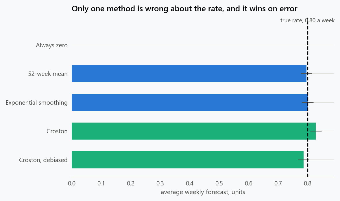
The true rate is 0.8 units a week, arriving in bursts. Any forecast that is honest about the average will be wrong every single week: too high on the 82 percent that are zero, too low on the 18 percent that are not. That is unavoidable, and it is why error scores behave so strangely here.
Five Methods and What the Scores Say
The candidates are: forecast zero, the mean of the last 52 weeks, exponential smoothing, Croston's method, and Croston with the standard debiasing factor. Croston's idea is to stop modelling the series directly and model two things instead, the size of a demand when it occurs and the gap between occurrences, updating each only when a demand arrives.
1
2
3
4
5
6
7
8
9
10
11
12
13
14
15
16
17
18
19
20
21
22
23
24
25
26
27
28
29
30
31
32
33
34
35
36
37
38
39
40
41
42
43
44
45
46
47
48
49
50
51
52
53
54
55
56
57
58
59
60
61
62
63
def forecast_zero(y, t, **kw):
    return 0.0


def forecast_mean(y, t, window=52, **kw):
    return y[max(0, t - window):t].mean()


def forecast_ses(y, t, alpha=0.1, **kw):
    f = y[:WARMUP].mean()
    for v in y[WARMUP:t]:
        f = alpha * v + (1 - alpha) * f
    return f


def croston(y, t, alpha=0.1, debias=False, **kw):
    """Smooth the demand size and the gap between demands separately."""
    nz = np.flatnonzero(y[:t])
    if nz.size < 2:
        return y[:t].mean()
    z = y[nz[0]]                                   # size estimate
    x = float(nz[0] + 1)                           # interval estimate
    last = nz[0]
    for i in nz[1:]:
        z = alpha * y[i] + (1 - alpha) * z
        x = alpha * (i - last) + (1 - alpha) * x
        last = i
    rate = z / x
    return rate * (1 - alpha / 2) if debias else rate


METHODS = {
    "always zero": (forecast_zero, {}),
    "52-week mean": (forecast_mean, {}),
    "exponential smoothing": (forecast_ses, {"alpha": 0.1}),
    "Croston": (croston, {"alpha": 0.1}),
    "Croston, debiased": (croston, {"alpha": 0.1, "debias": True}),
}


def evaluate(runs=200):
    out = {k: {"bias": [], "mae": [], "rmse": [], "f": []} for k in METHODS}
    for r in range(runs):
        y = series(T, rng=np.random.default_rng(100 + r))
        for name, (fn, kw) in METHODS.items():
            preds = np.array([fn(y, t, **kw) for t in range(WARMUP, T)])
            actual = y[WARMUP:T]
            out[name]["bias"].append(np.mean(preds - actual))
            out[name]["mae"].append(np.mean(np.abs(preds - actual)))
            out[name]["rmse"].append(np.sqrt(np.mean((preds - actual) ** 2)))
            out[name]["f"].append(preds.mean())
    return out


res = evaluate()
for name in METHODS:
    d = res[name]
    print(f"{name:22s} forecast {np.mean(d['f']):6.3f}  bias {np.mean(d['bias']):+7.4f}  "
          f"MAE {np.mean(d['mae']):6.3f}  RMSE {np.mean(d['rmse']):6.3f}")
best_mae = min(METHODS, key=lambda k: np.mean(res[k]["mae"]))
best_rmse = min(METHODS, key=lambda k: np.mean(res[k]["rmse"]))
print(f"lowest MAE:  {best_mae}")
print(f"lowest RMSE: {best_rmse}")
| Method | Average forecast | Bias | Mean absolute error | Root mean squared error |
|---|---|---|---|---|
| Always zero | 0.000 | −0.7951 | 0.795 | 1.942 |
| 52-week mean | 0.795 | −0.0006 | 1.274 | 1.789 |
| Exponential smoothing | 0.795 | −0.0002 | 1.276 | 1.818 |
| Croston | 0.829 | +0.0340 | 1.295 | 1.783 |
| Croston, debiased | 0.788 | −0.0074 | 1.270 | 1.781 |
The lowest mean absolute error belongs to the forecast of zero, by a wide margin, and it is the only method with a large bias. That is not a quirk of this simulation: the absolute error is minimised by the median of the distribution, and when 82 percent of weeks are zero, the median is zero. Any evaluation that ranks by mean absolute error on an intermittent series will choose a forecast that orders nothing.
The squared error behaves better, because it is minimised by the mean, and it ranks the debiased Croston forecast first. But the four sensible methods are separated by two percent on that score, which is not a margin anyone should act on.
The bias column shows Croston's known flaw. Estimating a rate as size divided by interval overstates it, because the expectation of a ratio is not the ratio of expectations, and the standard correction multiplies by one minus half the smoothing constant. Here that moves the forecast from 0.829 to 0.788 against a truth of 0.8, turning a 3.6 percent overstatement into a 1.5 percent understatement.
Judging the Forecast by the Decision
The forecast exists to set a stock level. That is the comparison that separates these methods, and it needs the ordering rule written down: review every week, order up to a level proportional to the forecast over the lead time, and count the share of demand filled from stock.
1
2
3
4
5
6
7
8
9
10
11
12
13
14
15
16
17
18
19
20
21
22
23
24
25
26
27
28
29
30
31
32
33
34
35
36
37
38
39
40
41
42
43
44
45
46
47
48
49
50
51
52
53
LEAD = 2


def run_inventory(y, preds, multiplier, lead=LEAD):
    """Order up to a level set from the forecast; count demand met from stock."""
    on_hand = preds[0] * (lead + 1) * multiplier
    pipeline = [0.0] * lead
    met = short = 0.0
    stock = []
    for i, (demand, f) in enumerate(zip(y, preds)):
        on_hand += pipeline.pop(0)
        served = min(on_hand, demand)
        met += served
        short += demand - served
        on_hand -= served
        stock.append(on_hand)
        target = f * (lead + 1) * multiplier
        position = on_hand + sum(pipeline)
        pipeline.append(max(0.0, target - position))
    return met / (met + short), np.mean(stock)


# Precompute one set of forecasts per method per series, then vary the stock rule.
SERIES = [series(T, rng=np.random.default_rng(500 + r)) for r in range(60)]
PREDS = {name: [np.array([fn(y, t, **kw) for t in range(WARMUP, T)]) for y in SERIES]
         for name, (fn, kw) in METHODS.items()}


def fill_and_stock(name, mult):
    fills, stocks = [], []
    for y, preds in zip(SERIES, PREDS[name]):
        fill, stock = run_inventory(y[WARMUP:T], preds, mult)
        fills.append(fill)
        stocks.append(stock)
    return np.mean(fills), np.mean(stocks)


TARGET = 0.95
for name in METHODS:
    if name == "always zero":
        print(f"{name:22s} fill rate 0.0% at any multiplier, because it never orders")
        continue
    lo, hi = 0.5, 20.0
    for _ in range(30):
        mid = (lo + hi) / 2
        if fill_and_stock(name, mid)[0] < TARGET:
            lo = mid
        else:
            hi = mid
    mult = (lo + hi) / 2
    fill, stock = fill_and_stock(name, mult)
    print(f"{name:22s} needs multiplier {mult:4.2f} for {fill:5.1%} fill, "
          f"holding {stock:5.2f} units on average")
| Method | Multiplier for a 95% fill rate | Average stock held |
|---|---|---|
| Always zero | never orders, fill rate 0% | 0 |
| 52-week mean | 3.69 | 7.81 units |
| Exponential smoothing | 3.02 | 8.60 units |
| Croston | 3.39 | 7.08 units |
| Croston, debiased | 3.57 | 7.08 units |
Now the methods separate in a way that means something. At the same service level, the Croston forecasts hold 7.08 units against 7.81 for the rolling mean and 8.60 for exponential smoothing: nine and eighteen percent less stock for the same promise to the customer. That ranking is invisible in the error table, where these methods differed by two percent and in the opposite order for absolute error.
Exponential smoothing does worst because it reacts to individual weeks. After a demand it raises the forecast and orders more; after a run of zeros it lowers the forecast and lets stock run down, which is precisely backwards for a series where demand arrives at random. Croston updates only when something happens, so its level is steadier and the stock it implies is steadier too.
The two Croston rows land on identical stock at different multipliers, which is worth understanding rather than glossing. Debiasing scales every forecast by a constant, and the tuned multiplier scales it back, so under a rule calibrated to a service level a constant bias factor cancels. The correction matters when the forecast is used as an expected value in its own right, for budgeting, for capacity planning or for any comparison against a target, and not when it feeds a rule whose scale is fitted anyway.
What Is Actually Being Predicted
There is a deeper point behind the metrics. A one-step forecast of 0.8 units for a week that will contain either zero or five units is not a prediction of the week; it is a statement about the rate. The useful outputs of an intermittent model are not point forecasts at all: the probability of any demand in the next $k$ weeks, the distribution of demand over the lead time, and the quantile of that distribution corresponding to the service level.
Evaluating those requires distributional scores rather than error metrics. When the pipeline cannot support that, the fallback used here is nearly as good and much simpler: run the candidate forecasts through the decision rule they feed and compare the cost of the outcome.
What to Do
- Never rank intermittent forecasts by mean absolute error or any percentage error. The first selects a forecast of zero and the second is undefined on most weeks.
- Check the bias of the average forecast against the long-run rate. It is the one error score that still means what it says on these series.
- Use Croston's method or one of its variants rather than smoothing the raw series. It updates on events instead of on the calendar, which is what the demand does.
- Apply the debiasing factor when the forecast is read as an expected value, and understand that it cancels when the forecast only sets the scale of a rule tuned to a service level.
- Evaluate on the decision: stock needed for a target fill rate, cost of stockouts, or whatever the forecast actually drives. That comparison separated methods that the error table ranked as equivalent.
- Report the probability of demand and a lead-time distribution where the tooling allows, rather than a point forecast that will be wrong in every single week by construction.
The figure generator in the blog-reproducibility repository reproduces this article's figure; run it with --dry-run to print the numbers behind the figure without writing an image.
References
- Croston, J. D. (1972). Forecasting and stock control for intermittent demands. Operational Research Quarterly, 23(3), 289-303.
- Syntetos, A. A., & Boylan, J. E. (2005). The accuracy of intermittent demand estimates. International Journal of Forecasting, 21(2), 303-314.
- Syntetos, A. A., Boylan, J. E., & Croston, J. D. (2005). On the categorization of demand patterns. Journal of the Operational Research Society, 56(5), 495-503.
- Teunter, R. H., Syntetos, A. A., & Babai, M. Z. (2011). Intermittent demand: linking forecasting to inventory obsolescence. European Journal of Operational Research, 214(3), 606-615.
- Kourentzes, N. (2014). On intermittent demand model optimisation and selection. International Journal of Production Economics, 156, 180-190.
- Hyndman, R. J., & Koehler, A. B. (2006). Another look at measures of forecast accuracy. International Journal of Forecasting, 22(4), 679-688.
Embed interactive plots, widgets, and demos using <figure>, <iframe>, or <div class="interactive-embed"> containers. Ensure each embed includes descriptive captions for accessibility.
How to cite
Use the quick export buttons to save citations for reference managers or copy the formatted text directly.
Diogo Ribeiro (2026). Intermittent Demand: Forecasting a Series That Is Mostly Zeros. Faculty of Media Arts and Design, Technical University of Porto. https://diogoribeiro7.github.io/statistics/intermittent_demand_forecasting_mostly_zeros/.

