Topics
An engineer has three years of hourly peak load on a piece of equipment and has to say what load it should be rated for over the next ten years. The worst hour on record was 265. Three answers are offered: rate it for 265 plus a margin; fit a normal distribution and read off a high quantile; or say that the data cannot answer a question about events rarer than the record. The first two are wrong in different directions, and the third is too pessimistic, because the shape of a tail can be estimated from the observations that are already in it.
The Maximum Reaches as Far as the Record
The largest of $n$ observations sits near the quantile $1 - 1/n$. Three years of hourly data is 26,280 observations, so the sample maximum estimates the level exceeded about once in three years. The ten-year level is three times rarer than anything in the record; the hundred-year level, thirty times rarer. Neither is in the data, and any estimate of either is an extrapolation.
It is also a noisy one. The probability that a three-year record contains at least one event of the ten-year kind is very nearly $1 - e^{-0.3}$, about 26 percent. One record in four contains something rarer than its own length and overstates the three-year level; three in four do not and understate anything beyond it. Adding a fixed margin to the maximum does not repair this, because the right margin depends on how fast the tail thins out, which is exactly what has not been estimated.
Fitting a familiar distribution to the whole dataset is worse. The body of the data determines the fit, and the body says nothing about the tail. A normal distribution fitted to heavy-tailed data reports a ten-year level that the record has already exceeded many times.
What the Theory Provides
Extreme value theory rests on a limit result about the shape of tails. For a wide class of distributions, the excess over a high threshold $u$, conditional on exceeding it, approaches a generalised Pareto distribution as the threshold rises:
The scale $\sigma$ sets the size of typical excesses. The shape $\xi$ sets how the tail decays: $\xi > 0$ is a power-law tail with no upper limit and rare events far larger than typical ones, $\xi = 0$ is an exponential tail, and $\xi < 0$ is a tail with a finite upper bound. The shape is the quantity a margin would need to know and does not.
With $\zeta_u$ the fraction of observations above the threshold and $H$ observations per year, the level exceeded on average once in $T$ years is
The three parameters are estimated from every observation above the threshold, typically hundreds of points, rather than from the single largest one. That is the whole advantage: the tail's shape is read from the part of the tail that has been observed, and used to extend it.
A Three-Year Record
The simulated load has a Student-t tail with four degrees of freedom, which is heavy, with a true shape of $\xi = 0.25$, and has closed-form quantiles, so the true return levels are known.
1
2
3
4
5
6
7
8
9
10
11
12
13
14
15
16
17
18
19
20
21
22
23
24
25
26
27
28
29
30
31
32
33
34
35
36
37
38
39
40
import numpy as np
from scipy import stats

rng = np.random.default_rng(0)
df, loc, scale = 4, 100.0, 10.0
H = 8760                                   # hours per year
n = 3 * H                                  # three years of hourly peak load
x = loc + scale * rng.standard_t(df, n)

def true_level(T):                          # level exceeded once per T years, on average
    return loc + scale * stats.t.ppf(1 - 1 / (T * H), df)
print(f"true levels: 3-year {true_level(3):.0f}, 10-year {true_level(10):.0f}, "
      f"100-year {true_level(100):.0f}")
print(f"sample max {x.max():.0f}, max + 20% {1.2*x.max():.0f}")
mu, sd = x.mean(), x.std()
print(f"normal fit: 10-year {mu + sd*stats.norm.ppf(1-1/(10*H)):.0f}, "
      f"100-year {mu + sd*stats.norm.ppf(1-1/(100*H)):.0f}")

def pot(x, q):
    u = np.quantile(x, q)
    exc = x[x > u] - u
    xi, _, sigma = stats.genpareto.fit(exc, floc=0)
    zeta = np.mean(x > u)
    level = lambda T: u + sigma / xi * ((T * H * zeta) ** xi - 1)
    return u, exc, xi, sigma, zeta, level

u, exc, xi, sigma, zeta, level = pot(x, 0.98)
print(f"\nPOT at 98th percentile: u = {u:.1f}, {len(exc)} exceedances, "
      f"xi = {xi:.2f} (true {1/df}), sigma = {sigma:.1f}")
print(f"GPD return levels: 10-year {level(10):.0f}, 100-year {level(100):.0f}")

r = np.random.default_rng(1)
boot = []
for _ in range(500):
    xb = x[r.integers(0, n, n)]
    *_, lv = pot(xb, 0.98)
    boot.append((lv(10), lv(100)))
boot = np.array(boot)
print("bootstrap 90% CI: 10-year [{:.0f}, {:.0f}], 100-year [{:.0f}, {:.0f}]".format(
    *np.percentile(boot[:, 0], [5, 95]), *np.percentile(boot[:, 1], [5, 95])))
| Estimate of the ten-year level | Value |
|---|---|
| True | 326 |
| Sample maximum (three years) | 265 |
| Sample maximum plus 20 percent | 318 |
| Normal fit | 159 |
| Generalised Pareto, threshold at the 98th percentile | 302, 90% interval 255 to 355 |
For the hundred-year level the truth is 502, the normal fit says 166, and the Pareto fit says 425 with an interval from 319 to 563.
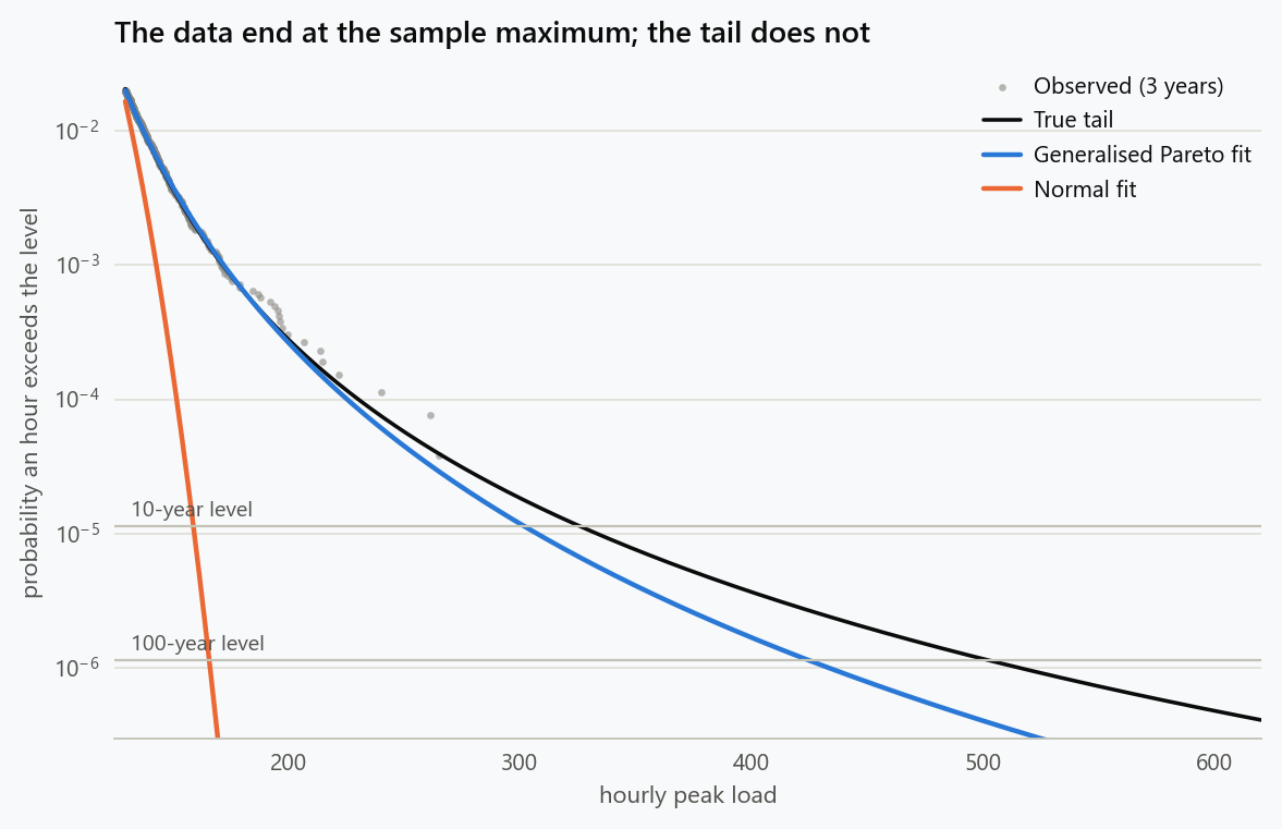
The picture is the argument. The observed points stop at the sample maximum, a little below the three-year line. The normal fit leaves the data before the 98th percentile, and at the level it calls a ten-year event the true exceedance probability is roughly 180 times what it claims. The Pareto fit follows the observed tail through 526 exceedances and continues along the true curve to levels three and thirty times rarer than anything observed.
Two features of the result deserve attention. The fit is a little low: the estimated shape is 0.19 against a true 0.25, and the ten-year estimate is 7 percent under the truth. And the intervals are wide and asymmetric, the hundred-year interval spanning almost a factor of two. Neither is a defect. The first is the threshold bias discussed next; the second is what the uncertainty about a hundred-year event from a three-year record actually is, and an estimate that reported it narrower would be lying.
Choosing the Threshold
The Pareto form is a limit, exact only as the threshold goes to infinity. A low threshold gives many exceedances and a biased shape, because the tail has not yet settled into its limiting form. A high threshold gives an unbiased shape estimated from too few points.
1
2
3
4
print("quantile   u      exceedances   xi     100-year level")
for q in (0.90, 0.95, 0.98, 0.99, 0.995):
    u_, exc_, xi_, s_, z_, lv_ = pot(x, q)
    print(f"{q:<10}{u_:6.1f}{len(exc_):>10}{xi_:>10.2f}{lv_(100):>12.0f}")
| Threshold quantile | Exceedances | Shape $\xi$ | Hundred-year level |
|---|---|---|---|
| 90% | 2,628 | 0.16 | 373 |
| 95% | 1,314 | 0.20 | 440 |
| 98% | 526 | 0.19 | 425 |
| 99% | 263 | 0.22 | 471 |
| 99.5% | 132 | 0.28 | 564 |
The shape rises with the threshold, though not steadily, from 0.16 to 0.28 against a true value of 0.25, and the hundred-year estimate moves with it, from 373 to 564 around a truth of 502. The two standard diagnostics for picking a threshold both come from the Pareto property itself. Above a valid threshold the mean excess is linear in the threshold, so a plot of mean excess against threshold should turn straight; and the shape estimate should stop changing, so a plot of $\xi$ against threshold should go flat. In practice the choice lands between the 90th and 99th percentiles, and the honest report is not one number but the range across a few thresholds, which here is the range the truth sits inside.
Repeating the Experiment
One dataset shows one outcome. Two hundred simulated three-year records show the distribution of each method's ten-year estimate.
| Method | Median estimate | Interquartile range | Share below the truth |
|---|---|---|---|
| Sample maximum | 291 | 255 to 333 | 72% |
| Sample maximum plus 20% | 350 | 307 to 400 | 38% |
| Normal fit | 160 | 159 to 160 | 100% |
| Generalised Pareto, 98% threshold | 313 | 289 to 344 | 62% |
The truth is 326. The normal fit is precisely and confidently wrong: an interquartile range of one unit around a value half the true level, because the body of the data pins down the mean and standard deviation and neither has anything to do with the tail. The sample maximum is biased low and spread widely. The margin of 20 percent happens to bracket the truth for this tail, and that is luck: for an exponential tail the same margin would be far too generous and for a heavier one far too little, and nothing in the procedure tells the engineer which tail they have. The Pareto estimate is tighter than the maximum, less biased, and comes with an interval; its remaining downward bias is the threshold effect, and it shrinks at higher thresholds at the cost of width.
The shape parameter is also what tells the engineer how the risk scales. With $\xi = 0.25$, going from the ten-year to the hundred-year level multiplies the excess over the 98th-percentile threshold by about 1.9, tending to $10^{0.25}$, a factor of 1.8, for longer return periods. With an exponential tail it would add a constant instead. For this tail the hundred-year level sits 54 percent above the ten-year level; for an exponential tail with the same scale it would sit about 7 percent above. Which of those margins applies is not visible in the sample maximum.
Exceedances Come in Clusters
Real load series are dependent in time. A hot afternoon is followed by another, a congestion event lasts hours, a bearing that runs hot stays hot. Exceedances then arrive in clusters, and the count of exceedances overstates the amount of independent information about the tail.
1
2
3
4
5
6
7
8
9
10
11
12
13
14
15
16
17
18
19
20
21
22
phi = 0.8
z = np.empty(n)
z[0] = rng.normal()
eps = rng.normal(size=n)
for t in range(1, n):
    z[t] = phi * z[t - 1] + np.sqrt(1 - phi**2) * eps[t]
xd = loc + scale * stats.t.ppf(stats.norm.cdf(z), df)   # same t4 marginal, dependent in time

ud = np.quantile(xd, 0.98)
over = xd > ud
clusters, gap = 0, 10**9
for t in range(n):                       # a new cluster starts after 24 hours below threshold
    if over[t]:
        if gap >= 24:
            clusters += 1
        gap = 0
    else:
        gap += 1
print(f"dependent series: {over.sum()} exceedances in {clusters} clusters, "
      f"extremal index ~ {clusters/over.sum():.2f}")
_, _, xi_d, sig_d, zeta_d, lv_d = pot(xd, 0.98)
print(f"naive POT on the dependent series: xi = {xi_d:.2f}, 10-year level {lv_d(10):.0f}")
The series has the same marginal distribution as before, so the true return levels are unchanged, but the process driving it has a lag-one correlation of 0.8. Its 526 exceedances fall into 194 clusters, an extremal index of about 0.37: each extreme event lasts, on average, close to three hours above the threshold. The naive fit still lands at a ten-year level of 303, because the marginal quantile is what it estimates and the marginal distribution has not changed. What has changed is the information behind it. The bootstrap interval computed by resampling hours treats 526 exceedances as independent when there are 194 events, and it comes out too narrow by roughly the square root of that ratio.
The standard remedy is to decluster: identify independent events with a run rule, keep the maximum of each cluster, fit the Pareto distribution to those, and use the cluster rate rather than the hourly exceedance rate in the return-level formula. The extremal index is worth reporting on its own. It is the number of independent extreme events per exceedance, and it is the honest denominator for how much the record actually says about the tail.
Non-stationarity is the other complication real series bring. Under a load trend or a seasonal cycle the ten-year level is not a constant, and the fit should let the scale or the threshold depend on time or on covariates, or be made separately by season. A single return level fitted to a trending series describes the average of a past that is not coming back.
Where It Shows Up
The setting in the example is equipment rating, and the same arithmetic governs every capacity or margin decision made from a finite record: the peak demand a substation must carry, the flood level a site must stay above, the request rate a service must absorb, the latency a service-level objective promises at the 99.99th percentile from a month of measurements, the operational loss a reserve must cover. In every case the record is shorter than the return period of the event being planned for, the sample maximum is the tempting number, and the question is the shape of the tail beyond it.
What to Do
- Do not read the tail from the sample maximum. It estimates the level at the length of the record and no further, and it is low three times out of four.
- Fit the exceedances above a high threshold to the generalised Pareto distribution and compute return levels from the fitted shape.
- Check a range of thresholds with the mean-excess and shape-stability plots, and report the range of return levels rather than one.
- Decluster dependent series and use the number of independent events, not the number of exceedances, as the basis for uncertainty.
- Report the interval as the deliverable. A hundred-year level from three years of data is uncertain by a factor approaching two, and a design margin should be set from the upper end of that interval, not from the point estimate.
- Model trends and seasons in the parameters when the series has them.
The tail cannot be seen in the data. Its shape can, and that is enough to say how far the tail goes with an honest statement of how sure one can be.
The figure generator in the blog-reproducibility repository reproduces this article's figure; run it with --dry-run to print the numbers behind the figure without writing an image.
References
- Coles, S. (2001). An Introduction to Statistical Modeling of Extreme Values. Springer.
- Pickands, J. (1975). Statistical inference using extreme order statistics. The Annals of Statistics, 3(1), 119-131.
- Balkema, A. A., & de Haan, L. (1974). Residual life time at great age. The Annals of Probability, 2(5), 792-804.
- Davison, A. C., & Smith, R. L. (1990). Models for exceedances over high thresholds. Journal of the Royal Statistical Society: Series B, 52(3), 393-442.
- Scarrott, C., & MacDonald, A. (2012). A review of extreme value threshold estimation and uncertainty quantification. REVSTAT Statistical Journal, 10(1), 33-60.
- Embrechts, P., Klüppelberg, C., & Mikosch, T. (1997). Modelling Extremal Events for Insurance and Finance. Springer.
- McNeil, A. J., Frey, R., & Embrechts, P. (2015). Quantitative Risk Management: Concepts, Techniques and Tools (2nd ed.). Princeton University Press.
Embed interactive plots, widgets, and demos using <figure>, <iframe>, or <div class="interactive-embed"> containers. Ensure each embed includes descriptive captions for accessibility.
How to cite
Use the quick export buttons to save citations for reference managers or copy the formatted text directly.
Diogo Ribeiro (2025). Extreme Value Theory: Estimating the Tail You Have Not Seen. Faculty of Media Arts and Design, Technical University of Porto. https://diogoribeiro7.github.io/statistics/extreme_value_theory_operational_risk/.

