Topics
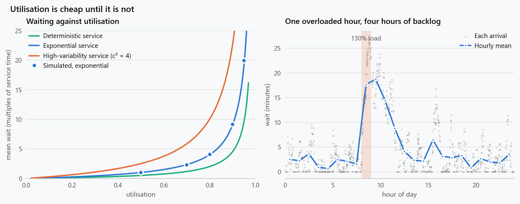
A maintenance crew is busy 85 percent of the time, and the planner wants 95, because idle technicians are waste. The ticket queue has other ideas. Every operation that serves arriving work meets the same fact eventually: waiting time is not proportional to load. It is nearly flat until utilisation reaches about 70 percent, bends sharply through 80, and goes vertical past 90. The formulas that describe this are a century old, short, and checked here by simulation, and the capacity decisions they imply are the opposite of the planner's instinct.
Little's Law
The one result that holds for any queue, whatever its arrival pattern or service rule, is Little's law: the average number of jobs in a system equals the arrival rate times the average time each spends there,
It is a conservation statement, not a model, and it lets one quantity be inferred from the other two. A repair shop that receives 40 jobs a day and holds 120 in progress has a lead time of three days, whatever anyone's tracking system says. Applied to the waiting line alone, it turns a mean wait into a mean backlog and back.
The Utilisation Curve
The simplest queue has one server, jobs arriving at random at rate $\lambda$, and service times that are random with mean $\tau$. Utilisation is $\rho = \lambda\tau$, the fraction of time the server is busy. When service times are exponentially distributed, the mean time a job waits before service starts is
At 50 percent utilisation a job waits one service time on average. At 80 percent, four. At 90, nine. At 95, nineteen. The denominator is what does the damage: each step toward full utilisation removes a slice of the slack that absorbed randomness, and the queue grows without bound as $\rho$ approaches one.
The simulation uses the Lindley recursion, which computes each job's wait from the previous job's wait, service time and the gap between arrivals, and applies to any arrival and service distributions.
1
2
3
4
5
6
7
8
9
10
11
12
13
14
15
16
17
18
19
20
21
22
23
24
25
26
27
28
29
30
31
32
import numpy as np
from math import factorial

def gg1_wait(arrivals, services):
    """Lindley recursion: waiting time in queue for a single FIFO server."""
    w = np.empty(len(services)); w[0] = 0.0
    for i in range(1, len(services)):
        w[i] = max(0.0, w[i-1] + services[i-1] - arrivals[i])
    return w

def ggc_wait(arrivals, services, c):
    """FIFO with c identical servers: each job takes the server that frees up first."""
    free = np.zeros(c); t = 0.0; w = np.empty(len(services))
    for i in range(len(services)):
        t += arrivals[i]
        k = np.argmin(free)
        start = max(t, free[k]); w[i] = start - t; free[k] = start + services[i]
    return w

rng = np.random.default_rng(0)
N = 200000
print("utilisation   simulated   formula rho/(1-rho)   95th percentile wait")
for rho in (0.5, 0.7, 0.8, 0.9, 0.95, 0.99):
    a = rng.exponential(1 / rho, N); s = rng.exponential(1.0, N)
    w = gg1_wait(a, s)[N // 10:]                   # drop the warm-up
    print(f"{rho:<13}{w.mean():>9.2f}{rho/(1-rho):>18.2f}{np.percentile(w, 95):>16.1f}")

rho = 0.8
a = rng.exponential(1 / rho, N); s = rng.exponential(1.0, N)
w = gg1_wait(a, s)
lam = 1 / a.mean()
print(f"Little's law at rho = 0.8: {lam:.3f} x {w.mean():.2f} = {lam * w.mean():.2f} jobs waiting on average")
| Utilisation | Mean wait, simulated | Mean wait, formula | 95th percentile wait |
|---|---|---|---|
| 0.50 | 1.02 | 1.00 | 4.7 |
| 0.70 | 2.30 | 2.33 | 8.6 |
| 0.80 | 4.09 | 4.00 | 14.3 |
| 0.90 | 9.15 | 9.00 | 30.0 |
| 0.95 | 19.96 | 19.00 | 63.1 |
| 0.99 | 66.85 | 99.00 | 208.5 |
All waits are in multiples of the mean service time. The simulation and the formula agree to within noise up to 95 percent. At 99 percent they do not, and the reason is itself a lesson: 200,000 jobs are not enough for a queue that close to saturation to settle into its long-run behaviour. A queue's memory is as long as its wait, and a real operation at 99 percent utilisation is never in steady state within a shift. It is always still recovering from the last surge.
Little's law checks out at 80 percent: an arrival rate of 0.802 times a mean wait of 3.98 gives 3.19 jobs waiting on average.
Variability Is the Other Half
Utilisation is not the only input. Two queues at the same utilisation can have waits that differ by a factor of five, and the difference is variability. Kingman's approximation for a single server makes the dependence explicit:
where $c_a$ and $c_s$ are the coefficients of variation of the times between arrivals and of the service times. The exponential case has $c_a^2 = c_s^2 = 1$ and the second factor is one, recovering the earlier formula.
1
2
3
4
5
6
7
8
print("rho = 0.8: service-time variability")
print("service distribution    c_s^2   simulated wait   Kingman approximation")
for name, sgen, cs2 in (("deterministic", lambda n: np.ones(n), 0.0),
                        ("exponential", lambda n: rng.exponential(1.0, n), 1.0),
                        ("lognormal, cv 2", lambda n: rng.lognormal(-0.5 * np.log(5), np.sqrt(np.log(5)), n), 4.0)):
    a = rng.exponential(1 / rho, N); s = sgen(N)
    w = gg1_wait(a, s)[N // 10:]
    print(f"{name:<23}{cs2:>5.1f}{w.mean():>17.2f}{rho/(1-rho) * (1 + cs2) / 2:>18.2f}")
| Service times at 80% utilisation | $c_s^2$ | Simulated mean wait | Kingman |
|---|---|---|---|
| Deterministic | 0 | 2.03 | 2.00 |
| Exponential | 1 | 4.10 | 4.00 |
| Lognormal, coefficient of variation 2 | 4 | 9.95 | 10.00 |
Same arrival process, same utilisation, same server. Making the service time perfectly regular halves the wait; making it highly variable, which is what a mix of five-minute resets and three-hour rebuilds looks like, multiplies it by two and a half. The arrival side behaves the same way: scheduled arrivals have $c_a^2$ near zero and walk-ins have it near one, which is why appointment systems exist.
The operational reading is that variability reduction and capacity are substitutes. A crew that standardises its work so that jobs take more predictable times gets the same reduction in waiting as a crew that adds capacity to bring utilisation from 80 percent down to about 67, and it gets it without hiring.
Pooling
Four crews, each with its own queue, each 80 percent busy. Or one queue feeding all four. Same people, same work, same utilisation.
1
2
3
4
5
6
7
8
9
10
11
12
def erlang_c(c, a):
    num = a**c / factorial(c) * c / (c - a)
    den = sum(a**k / factorial(k) for k in range(c)) + num
    return num / den

a = rng.exponential(1 / 0.8, N); s = rng.exponential(1.0, N)
print(f"four separate queues at rho = 0.8: mean wait {gg1_wait(a, s)[N//10:].mean():.2f}")
a4 = rng.exponential(1 / 3.2, N); s4 = rng.exponential(1.0, N)
w4 = ggc_wait(a4, s4, 4)[N//10:]
pw = erlang_c(4, 3.2)
print(f"one pooled queue, four servers: mean wait {w4.mean():.2f}  "
      f"(Erlang C: P(wait) = {pw:.2f}, mean wait {pw / (4 - 3.2):.2f})")
Separate queues: a mean wait of 3.95 service times. One pooled queue with four servers: 0.75, in agreement with the Erlang C formula, which puts the probability of waiting at all at 60 percent. That is a five-fold reduction from a change in routing alone.
The mechanism is that separate queues let a job wait at one crew while another crew stands idle. Pooling makes every idle server available to every waiting job, and the benefit grows with the number of servers pooled. The costs are real too: pooled servers need to be interchangeable, which fights specialisation; a shared queue may add travel or handoffs; and a pooled system fails all at once rather than one crew at a time. Where those costs are small, pooling is the cheapest capacity there is.
Recovering From an Overload
The utilisation curve describes steady state. Real load is not steady, and the queue integrates its history. A single hour at 130 percent load, in a day otherwise at 80 percent:
1
2
3
4
5
6
7
8
9
10
11
12
13
14
rng = np.random.default_rng(3)
hours, per_hour = 24, 60
rates = np.where(np.arange(hours) == 8, 1.3, 0.8)           # hour 8 runs at 130% load
a, s = [], []
for h in range(hours):
    n = rng.poisson(rates[h] * per_hour)
    a.append(np.sort(rng.uniform(h * per_hour, (h + 1) * per_hour, n)))
    s.append(rng.exponential(1.0, n))
arr = np.concatenate(a); srv = np.concatenate(s)
inter = np.diff(np.concatenate([[0.0], arr]))
w = gg1_wait(inter, srv)
for h in (7, 8, 9, 10, 11, 12, 14):
    m = (arr >= h * per_hour) & (arr < (h + 1) * per_hour)
    print(f"hour {h:>2}: load {rates[h]:.1f}, mean wait of arrivals that hour {w[m].mean():.1f} minutes")
| Hour | Load | Mean wait of jobs arriving that hour |
|---|---|---|
| 7 | 0.8 | 1.6 min |
| 8 | 1.3 | 17.7 min |
| 9 | 0.8 | 18.7 min |
| 10 | 0.8 | 14.4 min |
| 11 | 0.8 | 8.8 min |
| 12 | 0.8 | 4.1 min |
| 14 | 0.8 | 2.1 min |
Jobs arriving in the overloaded hour wait 18 minutes. So do jobs arriving in the hour after it, when the load is back to normal, and the backlog is still there at noon. The drain rate is the slack: at 80 percent utilisation the server clears the backlog at only 20 percent of its capacity, so the surplus of about 18 minutes' work that the hour leaves behind takes an hour and a half to remove in expectation, and with the randomness on top it is closer to four hours before waits return to normal. An average utilisation of 82 percent over the day describes none of this. The queue remembers peaks, and capacity has to be planned for them.
What the Averages Hide
The 95th percentile column in the first table is three times the mean at every utilisation. Waiting times are skewed: most jobs wait little and a few wait a long time, and the few are the ones that generate complaints, missed deadlines and escalations. A service target expressed as a mean is easy to meet while a fifth of jobs wait an unacceptable time. At 90 percent utilisation the mean wait is nine service times and the 95th percentile is thirty. Targets, and reports against them, belong on percentiles.
Where It Applies
The setting was a maintenance crew, and the same arithmetic governs any resource that serves arriving work: inference servers, where 90 percent GPU utilisation is a latency problem rather than an efficiency achievement; support desks; hospital beds and operating theatres; loading docks; build and test pipelines; call centres, which is where Erlang derived the pooled-queue formula in 1917. In each case there is a utilisation the operation can afford, given the wait it can tolerate and the variability it has, and it is rarely above 85 percent for a single server.
What to Do
- Measure three things, not one: utilisation, the variability of arrivals and the variability of service, since the wait depends on all of them.
- Set the utilisation target from the affordable wait, reading it off the curve for your variability, rather than from a headcount or efficiency rule.
- Reduce variability before adding capacity. Standardised work and scheduled arrivals move the curve down; they are cheaper than servers.
- Pool queues wherever the servers can be made interchangeable, and expect gains of several-fold at the same headcount.
- Plan capacity for peaks, because a queue integrates overloads and a busy hour costs an afternoon.
- Report and target percentiles, since the mean wait is met while the tail fails.
- Simulate the specific system, with its own arrival and service distributions, when a decision rides on the number. The recursion is six lines.
The figure generator in the blog-reproducibility repository reproduces this article's figure; run it with --dry-run to print the numbers behind the figure without writing an image.
References
- Little, J. D. C. (1961). A proof for the queuing formula L = λW. Operations Research, 9(3), 383-387.
- Kingman, J. F. C. (1961). The single server queue in heavy traffic. Mathematical Proceedings of the Cambridge Philosophical Society, 57(4), 902-904.
- Erlang, A. K. (1917). Solution of some problems in the theory of probabilities of significance in automatic telephone exchanges. Elektroteknikeren, 13, 5-13.
- Kleinrock, L. (1975). Queueing Systems, Volume 1: Theory. Wiley.
- Gross, D., Shortle, J. F., Thompson, J. M., & Harris, C. M. (2008). Fundamentals of Queueing Theory (4th ed.). Wiley.
- Hopp, W. J., & Spearman, M. L. (2011). Factory Physics (3rd ed.). Waveland Press.
Embed interactive plots, widgets, and demos using <figure>, <iframe>, or <div class="interactive-embed"> containers. Ensure each embed includes descriptive captions for accessibility.
How to cite
Use the quick export buttons to save citations for reference managers or copy the formatted text directly.
Diogo Ribeiro (2025). Queueing: Why 90 Percent Utilisation Means Waiting. Faculty of Media Arts and Design, Technical University of Porto. https://diogoribeiro7.github.io/mathematics/queueing_utilisation_waiting_time/.