Topics
The service desk replaced its ticket form in March. In April the share of calls handled in over thirty minutes fell from 18 percent to 15, and the operations review recorded an improvement. Nothing about the work had changed. The old form made agents type a duration, and they typed round numbers; the new one filled it in from the call timer.
Values entered by people cluster on multiples of five, ten, fifteen and sixty. It happens with durations, ages, weights, self-reported spend, story points and any estimate a human produces under mild time pressure. The clustering is called heaping, and it is harmless for some statistics and decisive for others.
Measuring How Much of It There Is
The simulation generates true handling times from a lognormal distribution with a median of eighteen minutes, then records them: a share of entries rounded to the nearest five minutes, the rest to the nearest minute. Whipple's index, borrowed from demography, measures how much mass sits on multiples of five. It reads 500 when every value is a multiple of five and, in its standard form, 100 when there is no preference; over the band from 10 to 60 used here, no preference reads about 108.
1
2
3
4
5
6
7
8
9
10
11
12
13
14
15
16
17
18
19
20
21
22
23
24
25
26
27
28
29
30
31
32
import numpy as np
from scipy import stats, optimize

RNG = np.random.default_rng(23)
N = 50_000
MU, SIGMA = np.log(18), 0.55      # true handling time, minutes


def record(n, heap, rng=RNG):
    """True durations, and what gets typed in: a share `heap` of entries are
    rounded to the nearest five minutes, the rest to the nearest minute."""
    true = rng.lognormal(MU, SIGMA, n)
    rounded5 = np.round(true / 5) * 5
    rounded1 = np.round(true)
    heaped = rng.random(n) < heap
    return true, np.where(heaped, rounded5, rounded1)


def whipple(v, lo=10, hi=60):
    """Whipple's index: how much of the mass sits on multiples of five.
    About 108 means no preference over 10 to 60 (100 in the standard index),
    500 means every value is a multiple of five."""
    band = v[(v >= lo) & (v <= hi)]
    on5 = np.isclose(band % 5, 0) | np.isclose(band % 5, 5)
    return 500 * on5.sum() / band.size


for heap in (0.0, 0.2, 0.5, 0.8, 1.0):
    _, obs = record(N, heap, rng=np.random.default_rng(2))
    share = np.isclose(obs % 5, 0).mean()
    print(f"heaped share {heap:4.0%}: values on a multiple of five {share:5.1%}, "
          f"Whipple index {whipple(obs):5.0f}")
| Share of entries rounded to five | Values on a multiple of five | Whipple index |
|---|---|---|
| 0% | 20.3% | 110 |
| 20% | 36.3% | 193 |
| 50% | 60.1% | 312 |
| 80% | 84.1% | 426 |
| 100% | 100.0% | 500 |
The index tracks the rounding almost linearly, which makes it a usable monitor in its own right: compute it per month, per team or per data source, and a jump means the recording behaviour changed. The first row reads 110 rather than exactly 100 mostly by arithmetic: the whole numbers from 10 to 60 include 11 multiples of five among 51, a little more than one in five, which alone gives 108. The lognormal shape, not perfectly flat across the band, adds about one point, and sampling noise the rest. Treat anything under about 110 as clean and anything over 150 as heavily rounded.
What Survives and What Does Not
1
2
3
4
5
6
for heap in (0.0, 0.2, 0.5, 0.8):
    true, obs = record(N, heap, rng=np.random.default_rng(3))
    print(f"heaped share {heap:4.0%}: mean {obs.mean():5.2f} (true {true.mean():5.2f})   "
          f"median {np.median(obs):5.2f} (true {np.median(true):5.2f})   "
          f"p90 {np.quantile(obs, 0.9):5.2f} (true {np.quantile(true, 0.9):5.2f})   "
          f"p99 {np.quantile(obs, 0.99):5.2f} (true {np.quantile(true, 0.99):5.2f})")
| Share rounded | Mean | True mean | Median | True median | p90 | True p90 | p99 | True p99 |
|---|---|---|---|---|---|---|---|---|
| 0% | 20.96 | 20.96 | 18.00 | 18.06 | 37.00 | 36.54 | 65.00 | 64.63 |
| 20% | 20.96 | 20.96 | 18.00 | 18.06 | 36.00 | 36.54 | 65.00 | 64.63 |
| 50% | 20.96 | 20.96 | 19.00 | 18.06 | 36.00 | 36.54 | 65.00 | 64.63 |
| 80% | 20.96 | 20.96 | 20.00 | 18.06 | 35.00 | 36.54 | 65.00 | 64.63 |
The mean is untouched to two decimal places at every level of rounding, because rounding to the nearest five is symmetric and the errors cancel. That is the reassuring half of the story, and it is why heaping so often goes unnoticed: the headline average is fine.
The quantiles are not fine. The median moves from 18 to 20 as rounding increases, an 11 percent error, because a quantile is a position in a sorted list and heaping moves the values around that position onto the nearest round number. The 90th percentile drifts the other way, down to 35. A percentile metric computed on heaped data is reporting the round number nearest the truth, not the truth.
A Threshold on a Round Number
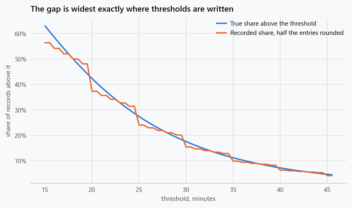
Thresholds are where this stops being academic. Service levels, escalation rules and alert conditions are written on round numbers, precisely the values that rounding piles mass onto.
1
2
3
4
5
6
true, obs = record(N, 0.5, rng=np.random.default_rng(5))
for thr in (25, 30, 35):
    print(f"threshold {thr}: truly over {np.mean(true > thr):6.2%}   "
          f"recorded strictly over {np.mean(obs > thr):6.2%}   "
          f"recorded at least {np.mean(obs >= thr):6.2%}   "
          f"sitting exactly on it {np.mean(obs == thr):5.2%}")
| Threshold | Truly over | Recorded strictly over | Recorded at least | Sitting exactly on the threshold |
|---|---|---|---|---|
| 25 minutes | 27.70% | 24.34% | 31.62% | 7.28% |
| 30 minutes | 17.79% | 15.63% | 20.31% | 4.67% |
| 35 minutes | 11.42% | 10.16% | 13.05% | 2.89% |
At thirty minutes the truth is 17.79 percent. A rule written as "over 30" reports 15.63 percent and a rule written as "30 or more" reports 20.31 percent. The gap between the two phrasings is 4.7 points, which is the mass piled exactly on the threshold, and it is larger than most of the changes these reports are built to detect. Two teams can compute the same metric from the same table, correctly, and differ by a quarter of its value.
Move the threshold off a round number and the problem disappears:
1
2
3
4
for thr in (27, 28, 32, 33):
    print(f"threshold {thr}: truly over {np.mean(true > thr):6.2%}   "
          f"recorded over {np.mean(obs > thr):6.2%}   "
          f"error {np.mean(obs > thr) - np.mean(true > thr):+6.2%}")
| Threshold | Truly over | Recorded over | Error |
|---|---|---|---|
| 27 minutes | 23.14% | 22.07% | −1.07% |
| 28 minutes | 21.14% | 21.10% | −0.03% |
| 32 minutes | 14.94% | 14.26% | −0.68% |
| 33 minutes | 13.69% | 13.63% | −0.06% |
The worst error here is one point and the typical one is a rounding artefact of the third decimal. A service level at 28 minutes is not meaningfully different from one at 30 as a commitment, and it is far better behaved as a measurement.
An Alarm With Nothing Behind It
The most expensive failure is not a biased number but a moving one. If the share of rounded entries changes, because a form changed, a team was retrained, or a new integration started filling the field automatically, every metric sensitive to heaping moves with it.
1
2
3
4
5
6
7
8
9
10
11
12
13
14
15
16
17
18
19
20
21
22
alarms = {"mean": 0, "median": 0, "p90": 0, "breach rate over 30": 0}
runs = 500
for i in range(runs):
    r = np.random.default_rng(1000 + i)
    _, before = record(8000, 0.30, rng=r)
    _, after = record(8000, 0.70, rng=r)          # same process, more rounding
    if abs(stats.ttest_ind(before, after, equal_var=False).pvalue) < 0.05:
        alarms["mean"] += 1
    if stats.mannwhitneyu(before, after).pvalue < 0.05:
        alarms["median"] += 1
    q_b, q_a = np.quantile(before, 0.9), np.quantile(after, 0.9)
    # Variance of a sample quantile is p(1-p) / (n f(q)^2); two of them for a difference.
    density = stats.gaussian_kde(before[:2000])(q_b)[0]
    se_q = np.sqrt(2 * 0.9 * 0.1 / (len(before) * density ** 2))
    if abs(q_a - q_b) > 1.96 * se_q:
        alarms["p90"] += 1
    p_b, p_a = np.mean(before > 30), np.mean(after > 30)
    se_p = np.sqrt(p_b * (1 - p_b) / len(before) + p_a * (1 - p_a) / len(after))
    if abs(p_a - p_b) > 1.96 * se_p:
        alarms["breach rate over 30"] += 1
for k, v in alarms.items():
    print(f"{k:22s} flags a change in {v / runs:5.1%} of runs, with no change in the work")
| Monitor | Flags a change |
|---|---|
| Mean | 4.4% |
| Median | 4.4% |
| 90th percentile | 50.6% |
| Breach rate over 30 minutes | 49.6% |
The underlying durations are drawn from the same distribution in both periods. Only the share of entries rounded to five minutes changes, from 30 percent to 70. The mean and median monitors behave: they fire at about the 5 percent rate their thresholds promise. The percentile monitor and the threshold monitor fire about half the time, and each one of those is an investigation that will find nothing, because there is nothing to find.
This is the mechanism behind the improvement in the introduction. It is also why "the metric moved when we changed the form" should be a standard hypothesis during any incident review of a moving metric.
Reading Rounded Values as What They Are
A value recorded as 30 by someone who rounds is not a claim that the duration was 30 minutes. It is a claim that it was somewhere near 30. Treating it that way, as an interval rather than a point, recovers the underlying distribution.
1
2
3
4
5
6
7
8
9
10
11
12
13
14
15
16
17
18
19
20
21
22
23
24
25
26
27
28
29
30
def fit_interval(obs):
    """Maximum likelihood for a lognormal when a value on a multiple of five
    only says the truth was within two and a half minutes of it."""
    on5 = np.isclose(obs % 5, 0)
    half = np.where(on5, 2.5, 0.5)
    lo = np.maximum(obs - half, 1e-6)
    hi = obs + half

    def nll(theta):
        mu, log_s = theta
        s = np.exp(log_s)
        p = stats.lognorm.cdf(hi, s, scale=np.exp(mu)) - stats.lognorm.cdf(lo, s, scale=np.exp(mu))
        return -np.log(np.clip(p, 1e-300, None)).sum()

    res = optimize.minimize(nll, [np.log(np.median(obs)), np.log(0.5)], method="Nelder-Mead")
    mu, s = res.x[0], np.exp(res.x[1])
    return mu, s


for heap in (0.2, 0.5, 0.8, 1.0):
    true, obs = record(N, heap, rng=np.random.default_rng(7))
    mu_hat, s_hat = fit_interval(obs)
    q = lambda p: stats.lognorm.ppf(p, s_hat, scale=np.exp(mu_hat))
    print(f"heaped share {heap:4.0%}: median {np.median(obs):5.2f} raw, {q(0.5):5.2f} fitted, "
          f"{np.median(true):5.2f} true   "
          f"p90 {np.quantile(obs, 0.9):5.2f} raw, {q(0.9):5.2f} fitted, "
          f"{np.quantile(true, 0.9):5.2f} true   "
          f"over 30 {np.mean(obs > 30):5.2%} raw, "
          f"{1 - stats.lognorm.cdf(30, s_hat, scale=np.exp(mu_hat)):5.2%} fitted, "
          f"{np.mean(true > 30):5.2%} true")
| Share rounded | Median raw | Median fitted | Median true | p90 raw | p90 fitted | p90 true | Over 30 raw | Over 30 fitted | Over 30 true |
|---|---|---|---|---|---|---|---|---|---|
| 20% | 18.00 | 17.96 | 17.94 | 36.00 | 36.15 | 36.27 | 16.28% | 17.36% | 17.56% |
| 50% | 18.00 | 17.95 | 17.94 | 35.00 | 36.18 | 36.27 | 15.49% | 17.38% | 17.56% |
| 80% | 20.00 | 17.95 | 17.94 | 35.00 | 36.21 | 36.27 | 14.62% | 17.41% | 17.56% |
| 100% | 20.00 | 17.94 | 17.94 | 35.00 | 36.22 | 36.27 | 14.01% | 17.42% | 17.56% |
Even when every single entry is rounded to five minutes, the fitted median is 17.94 against a truth of 17.94, and the fitted breach rate is 17.42 percent against a truth of 17.56, where the raw count says 14.01. The information survives rounding because the pattern of which round number each observation landed on still constrains the distribution; what is lost is only the last two and a half minutes of each value.
The cost is an assumption about shape. The fit above assumes a lognormal, which is reasonable for handling times and wrong for something bimodal. Check it before relying on it, by comparing the fitted curve against the recorded values away from the round numbers, where the data is not rounded and the fit has nothing to hide behind.
What to Do
- Compute a Whipple index, or simply the share of values on multiples of five and ten, for every human-entered numeric field. Do it per source and per month, because the interesting part is the change.
- Keep thresholds off round numbers. Twenty-eight minutes measures better than thirty, and it commits to the same thing.
- Write the comparison explicitly in the metric definition. "Over 30" and "30 or more" differ by the mass sitting exactly on the threshold, which here is nearly five points.
- Prefer the mean and other whole-distribution summaries when the field is heaped, and treat percentile metrics on those fields with suspicion.
- Add the recording path to the list of suspects whenever a monitored percentile or breach rate moves. A form change, a new integration or a retrained team will move them with no change in the underlying work.
- Fit rounded values as intervals when the number matters. It recovers the distribution almost exactly and costs a dozen lines.
The figure generator in the blog-reproducibility repository reproduces this article's figure; run it with --dry-run to print the numbers behind the figure without writing an image.
References
- Heitjan, D. F., & Rubin, D. B. (1990). Inference from coarse data via multiple imputation with application to age heaping. Journal of the American Statistical Association, 85(410), 304-314.
- Heitjan, D. F., & Rubin, D. B. (1991). Ignorability and coarse data. Annals of Statistics, 19(4), 2244-2253.
- Shryock, H. S., & Siegel, J. S. (1976). The Methods and Materials of Demography. Academic Press.
- Wang, H., & Heitjan, D. F. (2008). Modeling heaping in self-reported cigarette counts. Statistics in Medicine, 27(19), 3789-3804.
- Camarda, C. G., Eilers, P. H. C., & Gampe, J. (2008). Modelling general patterns of digit preference. Statistical Modelling, 8(4), 385-401.
- Crawford, S. L., Johannes, C. B., & Stellato, R. K. (2002). Assessment of digit preference in self-reported year at menopause: choice of an appropriate reference distribution. American Journal of Epidemiology, 156(7), 676-683.
Embed interactive plots, widgets, and demos using <figure>, <iframe>, or <div class="interactive-embed"> containers. Ensure each embed includes descriptive captions for accessibility.
How to cite
Use the quick export buttons to save citations for reference managers or copy the formatted text directly.
Diogo Ribeiro (2026). Digit Heaping: When Round Numbers Decide Who Breached the SLA. Faculty of Media Arts and Design, Technical University of Porto. https://diogoribeiro7.github.io/statistics/digit_heaping_rounded_entries_thresholds/.


