Topics
A social-media explanation of a scientific paper can be numerically accurate and still attach the wrong meaning to its most prominent number. Consider an imagined caption announcing that a result with a p-value below 0.05 has a 95% probability of being real. The caption appears to translate a technical statement into ordinary language, but it has changed the probability being discussed. The test concerns how a specified statistical procedure behaves under a model; the caption concerns whether a substantive claim is true after seeing the data. Moving between those questions requires information that the p-value does not contain. Neither an impressive graphic nor a link to a peer-reviewed paper supplies that information automatically.
The consequences extend beyond exaggerated certainty about one result. Two studies can be presented as contradictory because one crosses the conventional threshold and the other does not, even when their estimated effects are almost identical. A very small association can acquire the language of importance because it is measured precisely, while a potentially consequential association is dismissed because its uncertainty is large. These errors share a habit of replacing a quantitative argument with a categorical label. The label may accurately describe the outcome of a test, but the scientific conclusion still depends on the question, the measurement process, the magnitude of the estimate, and the other explanations that remain plausible.
The argument below develops those distinctions through explicit calculations. A synthetic population of studies will show how false-positive rates differ from the composition of selected results; a likelihood calculation will identify what is needed to assign probabilities to competing models; and two invented estimates will demonstrate how significance labels can manufacture the appearance of disagreement. These examples are mathematical constructions, not estimates of how much published science is correct. Their assumptions are deliberately simple so that each change in interpretation can be traced to a change in the quantity being calculated.
Archive note: dated 7 November 2024 for this collection; prepared and source-checked on 19 September 2026. The cited methodological sources were published before the archive date.
Begin with the probability that was actually calculated
Suppose a study estimates a mean difference, $\widehat\theta$, and that its sampling distribution is normal with known standard error $s$. The standard error describes how much the estimate varies across repeated studies using the specified design; it is not the standard deviation of individual observations. To test the null hypothesis $H_0:\theta=0$, define $Z=\widehat\theta/s$. Under the null and the rest of the model assumptions, $Z$ has a standard normal distribution. A prespecified two-sided test treats large positive and large negative values as departures from zero. Its p-value at the observed value $z$ is
where $\Phi$ is the standard normal cumulative distribution function. If the estimate is 0.20 and its standard error is 0.10, then $z=2$ and the two-sided p-value is approximately 0.0455. The calculation says that, under this null model, approximately 4.55% of repeated studies would produce a statistic at least as far from zero as the observed one. It does not say that the null model has probability 4.55%, or that the alternative has probability 95.45%. The null model is an input to the tail calculation. A probability assigned to that model after observing the statistic is a different output, requiring a different calculation.
The word “model” includes more than the assertion that the mean difference is zero. Normality of the estimator, the stated standard error, the sampling or randomisation design, and the procedure for deciding what to analyse all affect the reference distribution. If those assumptions misrepresent the analysis actually performed, the nominal p-value need not have the error properties attributed to it. A small value can therefore motivate scrutiny of the full statistical account without uniquely identifying which assumption is inadequate. The American Statistical Association's statement explicitly distinguishes p-values from probabilities of hypotheses and cautions against using a threshold as the sole basis for scientific conclusions.
A false-positive rate has a particular denominator
Consider a decision rule that rejects the null whenever the p-value is at most $\alpha=0.05$. For the continuous normal model above, its rejection threshold is approximately $|Z|\geq1.960$. Among repeated studies generated by the null model, the probability of rejection is 5%. This is the test's Type I error probability. Its denominator consists of null-generated studies, including those that do not reject. The question “What fraction of significant results came from null-generated studies?” has a different denominator: it starts with all the results that passed the selection rule, including those generated by an alternative. Reversing that conditioning is precisely where the missing information enters.
To make the distinction calculable, imagine 10,000 independent studies of equally precise contrasts. Suppose 90% are generated by $H_0$, under which $Z\sim\mathcal N(0,1)$, and 10% by a specified signal model $H_1$, under which $Z\sim\mathcal N(2,1)$. Here 2 measures the true contrast relative to its standard error. It is a signal-to-noise ratio for this study design, rather than a universal effect size or a claim that real effects take only two values. The 90:10 mixture is also stipulated. It defines the hypothetical population of questions entering the analysis and is not an empirical estimate for a scientific discipline.
The probability of rejection under $H_1$ is the test's power at this particular signal. With $c=\Phi^{-1}(1-\alpha/2)$, both tails must be included:
Thus approximately 51.60% of signal-generated studies reject. This definition counts rejection in either direction, including the very rare negative-tail rejection under the positive signal model; it does not silently redefine a two-sided test as a test for positive effects alone. Applying the null rejection rate and the signal rejection rate to their respective starting populations gives the following expected counts. They describe averages across repetitions of the synthetic collection, rather than exact counts that every collection must contain.
| Generating model | Studies entering the analysis | Expected rejections | Expected non-rejections |
|---|---|---|---|
| Null, $H_0$ | 9,000 | 450.0 | 8,550.0 |
| Signal, $H_1$ | 1,000 | 516.0 | 484.0 |
| Total | 10,000 | 966.0 | 9,034.0 |
Among the rejected studies, the probability that a study was generated by $H_1$ is approximately $516/(516+450)=0.5342$. The complementary probability is approximately 46.58%, even though the false-positive probability conditional on $H_0$ remains exactly 5%. These statements are consistent because their denominators differ. More generally, if $\pi$ is the starting probability of $H_1$ and $S$ denotes rejection, Bayes' rule gives
The formula identifies the information absent from the claim that a 5% test implies 95% reliable discoveries. We need the starting mixture and the rejection probability under the alternative, as well as the rejection probability under the null. In a real application, nonzero effects would usually vary in size, and power would have to be averaged over an appropriately justified alternative distribution. The calculation here supplies a counterexample to a universal interpretation; it does not supply a universal replacement percentage. These conditional probabilities can also be understood by selecting a study from the model population and learning whether its test rejected, without treating a ratio of two random realised counts as an exact identity in every finite collection.
A stricter threshold changes the selection, not the meaning of probability
Reducing the significance threshold changes both kinds of rejection. In the same 90:10 mixture, a threshold of 0.01 produces 90 expected null-generated rejections and approximately 282.4 signal-generated rejections. At 0.001, those expected counts become 9 and 98.4. The selected results contain a larger proportion of signal-generated studies, but many more signal-generated studies fail to pass. This tradeoff is a consequence of holding the design and the signal-to-noise ratio fixed while demanding a more extreme statistic. Improving measurement or increasing an informative sample could alter the design's power; changing the threshold alone does not provide that additional information.
| Threshold $\alpha$ | Power under $H_1$ | Expected null rejections | Expected signal rejections | $\Pr(H_1\mid S)$ |
|---|---|---|---|---|
| 0.05 | 51.60% | 450.0 | 516.0 | 53.42% |
| 0.01 | 28.24% | 90.0 | 282.4 | 75.83% |
| 0.001 | 9.84% | 9.0 | 98.4 | 91.62% |
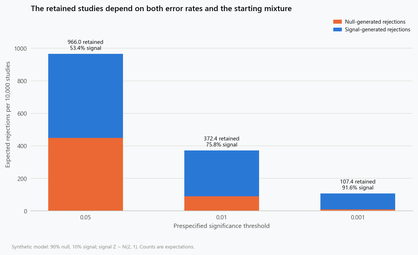
Original calculation for the stated model: 90% of studies have $Z\sim\mathcal N(0,1)$ and 10% have $Z\sim\mathcal N(2,1)$. The height of each bar is an expected count; its composition is conditional on the corresponding rejection rule.
The final row does not mean that a p-value of 0.001 universally confers 91.62% credibility. It concerns a result known only to have passed that threshold in one specified population of studies. Changing the prevalence of signal-generating questions, the sizes of the signals, or the analysis procedure changes the result. Nor does the table establish which threshold a particular scientific programme should choose. That decision depends on the consequences of missed effects and false claims, the resources available for follow-up, and the role of the test in a larger sequence of investigations. Error control is useful precisely when its scope is stated; a universal probability-of-truth interpretation obscures that scope.
The observed statistic carries information that a threshold discards
So far, the retained information has been the event $S$: the result was statistically significant. A paper that reports its estimate and standard error provides more information. In the two-model example, observing the signed statistic $z$ allows a comparison of the densities predicted by $H_1$ and $H_0$. Their likelihood ratio is
where $\phi$ is the standard normal density. At $z=2$, this ratio is $e^2\approx7.389$. The signal model assigns about 7.39 times as much density as the null model to that observed statistic. Since the statistic is continuous, the probability of an infinitely precise single value is zero; the density ratio is the relevant likelihood comparison and is also approached by the ratio of probabilities for the same shrinking interval around the observed value. It compares these two stipulated models. It does not establish that they exhaust the scientifically plausible explanations of the data.
To obtain a posterior model probability, combine the ratio with the starting probability $\pi$:
With $\pi=0.10$ and $z=2$, the posterior probability of $H_1$ is approximately 45.09%. With the same observed statistic, it becomes 6.95% when $\pi=0.01$ and 88.08% when $\pi=0.50$. The p-value remains 0.0455 in all three calculations because its null distribution and observed statistic have not changed. The posterior changes because the question asks how the observation updates different starting assessments within a specified comparison. Calling a p-value a probability that a claim is true would erase exactly the information responsible for those differences.
| Starting probability of $H_1$ | Two-sided p-value at $z=2$ | $\Pr(H_1\mid Z=2)$ |
|---|---|---|
| 1% | 0.0455 | 6.95% |
| 10% | 0.0455 | 45.09% |
| 50% | 0.0455 | 88.08% |
The 45.09% value also differs from the earlier 53.42% conditional on significance alone. There is no inconsistency: $Z=2$ and $|Z|\geq1.960$ are different information sets. The broader event pools values just beyond the cutoff with much larger values, along with the negative tail. The exact observation sits only slightly beyond the cutoff. Replacing a statistic by a binary label changes what has been learned and therefore changes the appropriate update. This is one reason to retain the estimate and its uncertainty when communicating a result, rather than reporting only that a threshold was crossed.
Direction supplies a further demonstration. At $z=-2$, the two-sided p-value is again 0.0455, but the likelihood ratio for the specified positive signal model against the null is $e^{-6}\approx0.00248$. This observation favours the null relative to that particular positive alternative, whereas $z=2$ favours the positive alternative. A negative-effect model could explain the negative observation better than either candidate, so this comparison does not certify the null as an adequate description. It shows that evidence for a particular explanation requires specifying that explanation. A Bayesian calculation also remains conditional on the chosen models and prior probabilities; replacing a p-value with a posterior number does not remove the obligation to justify the assumptions.
Two studies can disagree in label while agreeing closely in estimate
Consider a separate numerical example involving two independent studies of the same mean difference in the same units and target population. Study A estimates 0.20 with known standard error 0.10; Study B estimates 0.19 with known standard error 0.11. Their two-sided normal p-values are approximately 0.0455 and 0.0841. A threshold-based account might describe the first as confirming an effect and the second as failing to reproduce it. Yet the estimated differences are separated by only 0.01, and the second study is slightly less precise. The binary descriptions conceal those elementary quantitative facts.
Under the stated normal assumptions, the 95% confidence intervals are approximately [0.004, 0.396] for Study A and [−0.026, 0.406] for Study B. These intervals summarise uncertainty about each study's estimand under its sampling model. Their confidence level refers to the coverage of the interval-generating procedure over repeated samples, rather than assigning a 95% probability to a fixed parameter after the particular interval is observed. Neither interval implies that every included value is equally plausible. Their useful contribution here is to show the broad range of effects compatible with each estimate at the stated level, rather than converting the inclusion or exclusion of zero into another pair of categorical verdicts.
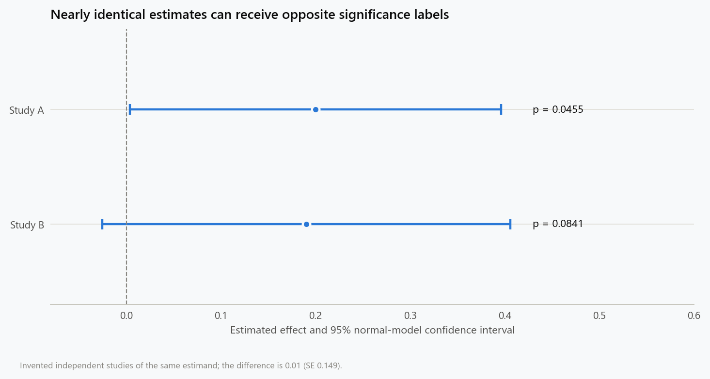
Original figure. Study A has standard error 0.10 and Study B has standard error 0.11. The plotted intervals use the known-standard-error normal model; these are invented estimates rather than results from a clinical or behavioural experiment.
A direct comparison addresses whether the underlying effects differ. Independence makes the variance of the difference equal to the sum of the two sampling variances, yielding
The resulting p-value for zero difference is approximately 0.946, and the 95% interval for the difference is approximately [−0.281, 0.301]. This calculation supplies little evidence of a discrepancy, while leaving considerable uncertainty about its magnitude. It does not prove that the two underlying effects are equal or sufficiently similar for a practical purpose. An equivalence claim would require a justified range of acceptably small differences and enough precision to assess it. If the studies shared participants or other sources of sampling variation, their covariance would also enter the comparison; adding variances without considering dependence would then be inappropriate. The distinction between comparing estimates and comparing significance labels is developed by Gelman and Stern.
Crossing the threshold again is another probability
Replication introduces an additional conditioning question. Return to the original synthetic model, with equal precision across studies and a fixed signal of two standard errors under $H_1$. If $H_1$ is known to generate the studies, a new independent study rejects with probability 0.5160, regardless of whether the previous independent study rejected. The first rejection does not change that generating model's fixed signal or its sampling variability. In this setting, an observed p-value below 0.05 cannot be interpreted as a 95% probability that a repeat study will cross the same threshold. Even when the signal model is known to hold, almost half of repeated studies do not reject under this design.
If the generating model is unknown and all we learn about the first study is that it rejected, the earlier mixture calculation assigns probability 0.5342 to $H_1$. A repeat study of the same question retains whichever generating model applied to the first; it does not draw a new model from the original 90:10 mixture. Conditional independence of its new sampling error then gives
The approximately 29.89% value is the probability of another two-sided rejection under this model and information set. It counts either tail, so it is not a probability of reproducing the estimated direction, obtaining a similar effect size, or replicating every substantive aspect of a scientific finding. Knowing the original signed statistic would lead to a different update, and changing the repeat study's sample size or measurement precision would change its rejection probability. The purpose of this calculation is to make those dependencies visible. A scientific assessment of replication needs to compare designs, populations, outcomes, effect estimates, and uncertainty, rather than replacing that assessment with whether two binary test decisions match.
The analysis procedure determines the reference probability
The preceding examples assume one prespecified test per study. Suppose instead that an investigator examines 20 independent outcomes, all generated under their respective null models, and reports whether any individual p-value is below 0.05. The probability that every test remains above the threshold is $0.95^{20}$, so the probability that at least one crosses it is
Every individual test can be correctly calibrated at 5% while this reporting procedure produces at least one nominally significant result in approximately 64.15% of repeated all-null collections. Reporting only the smallest p-value as though its test had been the sole planned comparison conceals the search that made an extreme result more likely. The exact percentage depends on independence; correlated outcomes require a different calculation. More generally, outcome definitions, exclusions, transformations, subgroups, and stopping decisions can create a collection of possible analyses that is not adequately represented by the reference distribution of one fixed test.
A prespecified multiplicity adjustment can change the relevant error guarantee. In this example, a Bonferroni threshold of $0.05/20=0.0025$ controls the probability of at least one false rejection at no more than 5% without requiring independence, provided each individual test is valid. With the additional independence assumption, the exact probability is approximately 4.883%. This is an error guarantee for a defined family of tests, not a posterior probability that each retained conclusion is correct. Choosing a family, an error criterion, and a correction requires scientific judgement about what decisions the analysis supports. Exploratory work can remain valuable when identified as exploratory and followed by a suitable confirmatory design; the problem is presenting a selected result as though the selection had never occurred.
The broader issue is transparency about the procedure that produced the number. A registered analysis plan, complete reporting of outcomes, and a reproducible record of deviations help readers understand which reference calculation is relevant. They do not make a poor measurement valid, remove all bias, or establish that a chosen outcome answers the substantive question. Greenland and colleagues emphasise that interpretation depends on the full set of statistical assumptions and on how analyses were selected for presentation. A public explanation should therefore describe the design and the scope of the analysis alongside its numerical result, rather than treating the p-value as an independent certification of scientific quality.
Effect size and scientific importance remain separate questions
The normal test statistic divides an estimate by its standard error. Consequently, an estimate of 0.002 with standard error 0.001 produces the same $z=2$ and p-value 0.0455 as an estimate of 2 with standard error 1. If these examples refer to the same outcome in the same units, their estimated magnitudes differ by a factor of 1,000 despite having identical p-values. Neither magnitude can be judged useful or harmful without substantive context, but the p-value cannot supply that judgement because it has combined magnitude and precision into a ratio. This also explains why changing measurement units consistently leaves the p-value unchanged: multiplying both the estimate and its standard error by the same positive conversion factor leaves the test statistic unchanged.
A reader evaluating a public scientific claim therefore needs the effect in interpretable units, the uncertainty around it, and a justification for why that effect would matter. For a risk claim, that may include the starting risk, the outcome definition, and the time window, as developed in the article on reading the starting risk before the percentage. For an association, it includes whether the design supports a causal interpretation. For an alleged failure to replicate, it includes a direct comparison of estimates and an account of relevant design differences. These are components of the inference, not optional background that becomes unnecessary once a small p-value appears.
The calculations also explain why abandoning one conventional cutoff would not, by itself, solve the communication problem. The same misunderstandings can be attached to a confidence interval, a posterior probability, a likelihood ratio, or a machine-learning score if the conditions that define it are omitted. Each quantity can answer a useful question, but the questions are not interchangeable. In the synthetic examples, a null tail probability, the composition of selected results, an update after an exact observation, and a repeat-study rejection probability all produce different numbers for coherent reasons. A responsible account states which question its number answers and what assumptions connect that answer to the scientific claim.
The most informative description of a study is consequently an argument about what was measured, how the observations constrain competing explanations, and what remains unresolved. A small p-value can be part of that argument when the test is appropriate and its scope is understood. It cannot substitute for the magnitude of an effect, the design needed to identify its cause, the probability model needed to compare hypotheses, or the body of evidence needed to assess a broader explanation. Communicating those distinctions preserves the useful role of statistical testing while preventing a numerical threshold from acquiring a meaning its calculation never established.
Reproducing the calculations
The calculation and figure script prints the rejection probabilities, expected counts, posterior updates, repeat-study probabilities, and study comparisons using the Python standard library. Run the following command from the reproducibility repository to reproduce the numerical results without writing files; omit the option to regenerate both figures with Matplotlib and the site's chart style. Independent checks compare the tail calculation with numerical integration, compare selected-study composition with simulated data, reconstruct posterior probabilities from weighted densities, and verify probability conservation and the repeated-study calculation. These checks establish consistency of the examples, while the article's explicit modelling assumptions determine the scope of their interpretation.
1
poetry run python scripts/figures/statistics/pvalue_evidence.py --dry-run
References
- Wasserstein, R. L., and Lazar, N. A. (2016). The ASA's statement on p-values: context, process, and purpose. The American Statistician, 70(2), 129–133.
- Greenland, S., Senn, S. J., Rothman, K. J., Carlin, J. B., Poole, C., Goodman, S. N., and Altman, D. G. (2016). Statistical tests, P values, confidence intervals, and power: a guide to misinterpretations. European Journal of Epidemiology, 31, 337–350.
- Gelman, A., and Stern, H. (2006). The difference between “significant” and “not significant” is not itself statistically significant. The American Statistician, 60(4), 328–331.
Embed interactive plots, widgets, and demos using <figure>, <iframe>, or <div class="interactive-embed"> containers. Ensure each embed includes descriptive captions for accessibility.
How to cite
Use the quick export buttons to save citations for reference managers or copy the formatted text directly.
Diogo Ribeiro (2024). Why a Small p-Value Does Not Settle a Scientific Claim. Faculty of Media Arts and Design, Technical University of Porto. https://diogoribeiro7.github.io/science-communication/why_a_small_p_value_does_not_settle_a_claim/.