Topics
A team reports 91.3 percent accuracy on a 400-case test set. A challenger model reaches 92.1 percent on the same cases, is declared better, and is deployed. The difference is 0.8 points. The standard error of an accuracy measured on 400 cases is about 1.5 points. The comparison was decided by noise, and no amount of care in training either model could have changed that, because the test set was never large enough to tell them apart.
Test-set size is usually set by convention, as 20 percent of whatever data exists. It should be set by the decision the test set has to support, and the arithmetic for that is short.
Accuracy Is a Proportion
A test-set accuracy is the fraction of $n$ cases the model gets right. It is a sample proportion, and a sample proportion has standard error $\sqrt{p(1-p)/n}$. For a model near 90 percent accuracy:
1
2
3
4
5
6
7
8
9
10
11
12
import numpy as np
from scipy import stats
from sklearn.metrics import roc_auc_score

rng = np.random.default_rng(0)

print("n      sd(points)  95% range of measured accuracy   CI half-width")
for n in (100, 400, 1000, 5000, 20000):
    acc = rng.binomial(n, 0.9, 20000) / n            # 20,000 test sets of size n
    lo, hi = np.percentile(acc, [2.5, 97.5]) * 100
    print(f"{n:<7}{acc.std()*100:>6.1f}      {lo:5.1f} to {hi:5.1f}"
          f"                {196*np.sqrt(0.09/n):5.1f}")
| Test cases | Spread of measured accuracy (sd, points) | Central 95% of measurements | 95% interval half-width |
|---|---|---|---|
| 100 | 3.0 | 84.0 to 95.0 | 5.9 |
| 400 | 1.5 | 87.0 to 92.8 | 2.9 |
| 1,000 | 0.9 | 88.1 to 91.8 | 1.9 |
| 5,000 | 0.4 | 89.2 to 90.8 | 0.8 |
| 20,000 | 0.2 | 89.6 to 90.4 | 0.4 |
The same model, evaluated on different 400-case test sets drawn from the same population, reports anything from 87 to 93 percent. A reported "91.3 percent" on 400 cases is the model's accuracy to within about three points, and the third significant figure is decoration. Halving the interval costs four times the cases.
The normal approximation behind $\sqrt{p(1-p)/n}$ is fine in the middle of the range. Near 0 or 1, and for small $n$, the Wilson interval is the one to report; it does not collapse to zero width when the model gets every case right.
The Minority Class Sets the Effective Size
Accuracy uses every case. Most metrics that matter use a subset, and the subset can be small even when the test set is not.
1
2
3
4
5
6
7
8
9
10
11
12
13
14
15
16
17
18
19
20
21
22
def bootstrap_ci(y, s, thr, B=1000):
    r = np.random.default_rng(1)
    out = []
    for _ in range(B):
        i = r.integers(0, len(y), len(y))
        yb, sb = y[i], s[i]
        if yb.sum() == 0:
            continue
        pred = sb > thr
        tp = (pred & (yb == 1)).sum()
        out.append((roc_auc_score(yb, sb), tp / max(pred.sum(), 1), tp / yb.sum()))
    return np.percentile(np.array(out), [2.5, 97.5], axis=0)

print("\nn = 5000; scores: positives N(1.5,1), negatives N(0,1); threshold 1.0")
print("prevalence  positives   AUC 95% CI          precision 95% CI     recall 95% CI")
for prev in (0.01, 0.10, 0.50):
    n = 5000
    y = (rng.uniform(size=n) < prev).astype(int)
    s = rng.normal(size=n) + 1.5 * y
    ci = bootstrap_ci(y, s, 1.0)
    print(f"{prev:<11.0%} {y.sum():<10}  [{ci[0,0]:.3f}, {ci[1,0]:.3f}]     "
          f"[{ci[0,1]:.2f}, {ci[1,1]:.2f}]         [{ci[0,2]:.2f}, {ci[1,2]:.2f}]")
| Prevalence | Positives in 5,000 | AUC 95% CI | Precision 95% CI | Recall 95% CI |
|---|---|---|---|---|
| 1% | 51 | 0.802 to 0.904 | 0.03 to 0.06 | 0.60 to 0.85 |
| 10% | 480 | 0.846 to 0.879 | 0.29 to 0.34 | 0.66 to 0.75 |
| 50% | 2,495 | 0.847 to 0.867 | 0.80 to 0.83 | 0.66 to 0.70 |
The scores come from the same distributions in all three rows, so the model is the same. Only the prevalence changes, and with it the number of positives. At 1 percent prevalence a 5,000-case test set contains 51 positives, the recall interval is 25 points wide, and the AUC interval spans a tenth of its range. The test set is large; the evaluation is not.
The rule that follows is that the effective size of a test set for recall is the number of positives, for precision the number of predicted positives, and for AUC something between the two, as Hanley and McNeil's formula for its variance makes explicit. For a recall interval of plus or minus 5 points at a recall near 0.8, the binomial formula asks for about 250 positives. At 1 percent prevalence that is a 25,000-case test set, and a team that budgeted 20 percent of a 10,000-row dataset has 20 positives, and a recall interval of about plus or minus 18 points.
Comparing Two Models
The most common use of a test set is not to measure one model but to choose between two, and the arithmetic changes in a way that helps.
Two models evaluated on the same cases make many of the same mistakes: the hard cases are hard for both. The difference in their accuracies is therefore far less variable than the difference between two independent measurements, and the relevant quantity is not $n$ but the number of cases on which the models disagree. A paired test uses this. McNemar's test looks only at the discordant cases, those one model gets right and the other wrong, and asks whether the split between them is even.
1
2
3
4
5
6
7
8
9
10
11
12
13
14
15
16
17
18
19
20
21
22
23
24
25
26
27
28
29
30
31
32
33
tau = 0.5
qA = stats.norm.ppf(0.90) * np.sqrt(1 + tau**2)
qB = stats.norm.ppf(0.91) * np.sqrt(1 + tau**2)

def draw(n, r):
    d = r.normal(size=n)                      # shared item difficulty
    a = d + r.normal(scale=tau, size=n) < qA  # model A correct?
    b = d + r.normal(scale=tau, size=n) < qB  # model B correct?
    return a, b

big = np.random.default_rng(30)
a, b = draw(200000, big)
d_rate, delta = np.mean(a != b), b.mean() - a.mean()
print(f"model A {a.mean():.3f}, model B {b.mean():.3f}, difference {delta:.4f}, "
      f"disagreement {d_rate:.3f}")

rng3 = np.random.default_rng(3)
reps = 2000
print("\nn       same set B>A   separate sets B>A   McNemar p<0.05   independent CIs disjoint")
for n in (200, 500, 1000, 2000, 5000, 10000, 20000):
    same = sep = mcn = disj = 0
    for _ in range(reps):
        a, b = draw(n, rng3)
        same += b.mean() > a.mean()
        a2, _ = draw(n, rng3)                     # A evaluated on its own test set
        sep += b.mean() > a2.mean()
        b_, c_ = np.sum(~a & b), np.sum(a & ~b)
        if b_ + c_ > 0:
            mcn += stats.binomtest(int(b_), int(b_ + c_)).pvalue < 0.05 and b_ > c_
        ha = 1.96 * np.sqrt(a.mean() * (1 - a.mean()) / n)
        hb = 1.96 * np.sqrt(b.mean() * (1 - b.mean()) / n)
        disj += (b.mean() - hb) > (a.mean() + ha)
    print(f"{n:<8}{same/reps:>10.0%}{sep/reps:>17.0%}{mcn/reps:>17.0%}{disj/reps:>20.0%}")
Model A has 90.0 percent accuracy and model B 90.9 percent, and they disagree on 8.4 percent of cases. Model B is genuinely better, by a margin that would matter in most applications.
| Test cases | Same set: B measures higher | Separate sets: B measures higher | Paired test significant | Independent intervals disjoint |
|---|---|---|---|---|
| 200 | 63% | 60% | 5% | 0% |
| 500 | 76% | 68% | 8% | 0% |
| 1,000 | 84% | 76% | 16% | 0% |
| 2,000 | 94% | 86% | 30% | 1% |
| 5,000 | 99% | 95% | 65% | 6% |
| 10,000 | 100% | 99% | 93% | 30% |
| 20,000 | 100% | 100% | 100% | 82% |
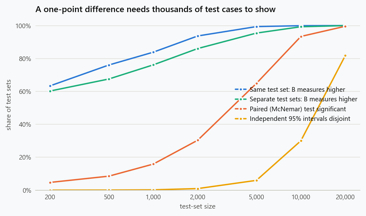
Four things are in that table. On 400 or 500 cases, the better model measures higher about three times in four, which means the worse model wins the comparison one time in four. Evaluating the two models on separate test sets, which happens whenever a challenger is scored on fresh data while the incumbent's number comes from its original evaluation, is worse at every size. The paired test needs between 5,000 and 10,000 cases to reach 80 percent power for a one-point difference. And the rule of thumb that two models differ when their confidence intervals do not overlap is so conservative that it needs 20,000 cases to fire reliably, because it ignores the pairing entirely and treats two correlated measurements as independent.
Sizing the Test Set
For a single metric with target half-width $E$ at 95 percent confidence:
with $p$ the expected value of the metric and $n$ counted in the units the metric is built from: cases for accuracy, positives for recall, predicted positives for precision.
For a paired comparison of two models with expected accuracy difference $\delta$ and disagreement rate $d$, McNemar's statistic under the alternative has mean $\sqrt{n}\,\delta/\sqrt{d}$, so for 80 percent power at a two-sided 5 percent level
1
2
3
4
5
6
7
8
n = int(round(7.85 * d_rate / delta**2))
r = np.random.default_rng(31)
hits = 0
for _ in range(reps):
    a, b = draw(n, r)
    b_, c_ = np.sum(~a & b), np.sum(a & ~b)
    hits += stats.binomtest(int(b_), int(b_ + c_)).pvalue < 0.05 and b_ > c_
print(f"formula size n = {n}, simulated power = {hits/reps:.0%}")
With $d = 0.084$ and $\delta = 0.0092$ the formula gives about 7,790 cases, and 7,734 from the unrounded simulated values the code uses. Simulating 2,000 test sets of 7,734 cases, the paired test rejects in 84 percent of them: the target, with a little margin from the difference between the normal approximation behind the formula and the exact binomial test being run.
The formula's inputs are more available than they look. The disagreement rate does not need labels: run both models on unlabeled production data and count how often they differ. A validation set gives a rough $\delta$. Both can be known before a single test case is labeled, which means the labeling budget can be set from the comparison it has to support rather than from a percentage.
Two consequences are worth drawing out. Models that disagree rarely are cheap to compare, since the discordant cases are the only ones that matter and few are needed. And a difference of a tenth of a point, which is the size of most improvements reported in leaderboard increments, needs a hundred times the cases of a one-point difference: with $d = 0.08$, about 630,000 of them.
Slices and Repeated Use
Two further ways a test set gets spent.
Slices. A 5,000-case test set reported across twenty segments has 250 cases per segment, and an interval of plus or minus 3.7 points on each segment's accuracy at 90 percent. The worst-performing segment in such a report is often the segment with the noisiest estimate, and the ranking of segments changes from one test set to the next. Segment-level claims need segment-level sizing, and the multiple-comparisons arithmetic applies to twenty intervals just as it does to twenty hypothesis tests.
Repeated looks. Every decision made by consulting the test set moves the chosen model toward the test set's particular noise. A test set used to pick among fifty configurations has become a validation set, and its final number is optimistic in the same way a winner's validation score is. Public leaderboards demonstrate this on every competition, where the private-set ranking reshuffles the public-set one. The protection is procedural: select on a validation set, and read the test set once, at the end, for the model already chosen. Where a test set has to be reused, the reusable-holdout results of Dwork and colleagues quantify how much each look costs and how to add noise so that the total stays bounded.
What to Do
- Compute the interval before reading the metric. Accuracy on $n$ cases has half-width about $1.96\sqrt{p(1-p)/n}$; a report without it is a point in a cloud of unknown size.
- Size by the minority class. For recall, count positives; for precision, count predicted positives. A rare-event test set needs to be large in proportion to its rarity.
- Compare models on the same cases with a paired test. Never compare a challenger's number on fresh data against an incumbent's number from an older evaluation.
- Size comparisons from the disagreement rate, measured on unlabeled data, using $n \approx 7.85\,d/\delta^2$ for 80 percent power.
- Report intervals for slices and expect the ranking of slices to move.
- Keep a final test set unread until one model has been chosen on the validation set.
The size of a test set is the resolution of every claim made from it. Choosing it by convention means choosing the resolution without looking.
The figure generator in the blog-reproducibility repository reproduces this article's figure; run it with --dry-run to print the numbers behind the figure without writing an image.
References
- Hanley, J. A., & McNeil, B. J. (1982). The meaning and use of the area under a receiver operating characteristic (ROC) curve. Radiology, 143(1), 29-36.
- Dietterich, T. G. (1998). Approximate statistical tests for comparing supervised classification learning algorithms. Neural Computation, 10(7), 1895-1923.
- McNemar, Q. (1947). Note on the sampling error of the difference between correlated proportions or percentages. Psychometrika, 12(2), 153-157.
- Brown, L. D., Cai, T. T., & DasGupta, A. (2001). Interval estimation for a binomial proportion. Statistical Science, 16(2), 101-133.
- Dwork, C., Feldman, V., Hardt, M., Pitassi, T., Reingold, O., & Roth, A. (2015). The reusable holdout: preserving validity in adaptive data analysis. Science, 349(6248), 636-638.
- Raschka, S. (2018). Model evaluation, model selection, and algorithm selection in machine learning. arXiv:1811.12808.
Embed interactive plots, widgets, and demos using <figure>, <iframe>, or <div class="interactive-embed"> containers. Ensure each embed includes descriptive captions for accessibility.
How to cite
Use the quick export buttons to save citations for reference managers or copy the formatted text directly.
Diogo Ribeiro (2025). How Big Does a Test Set Need to Be?. Faculty of Media Arts and Design, Technical University of Porto. https://diogoribeiro7.github.io/machine-learning/test_set_size_model_evaluation/.


