Topics
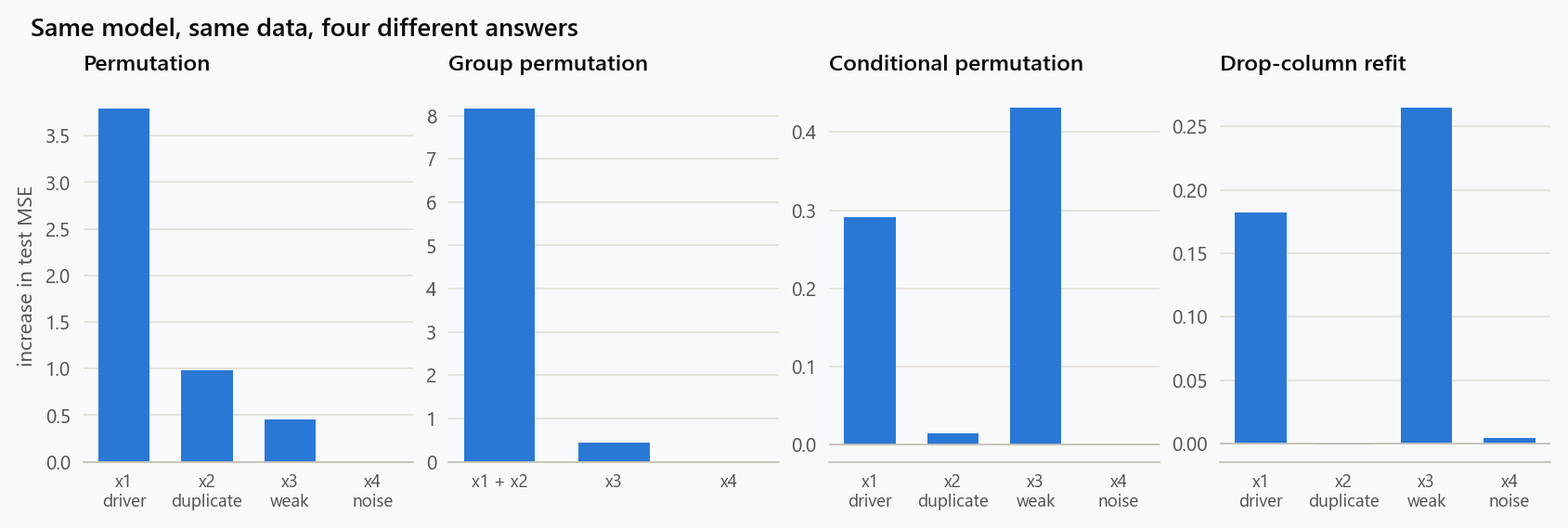
Someone asks which sensors matter. The answer is a bar chart from permutation importance: shuffle each column, see how much the error rises, rank. It is model-agnostic, cheap, and available in one function call. With correlated inputs it can put a sensor that does nothing above one that drives the outcome, while stripping the real driver of a third of its score. None of that is a bug.
What Permutation Importance Measures
Permuting a column breaks its relationship with the target and with every other column, then measures how much worse the fitted model does. The number means "how much this model's predictions degrade when this column becomes noise while everything else stays as it was."
Three consequences follow. It is a property of the fitted model, not of the data: a different model, or the same model trained with another seed, gives a different answer. If another column carries the same information, the model may lean on either, so the score is split between them and part of it disappears, because shuffling one leaves the other to cover. And shuffling one of two correlated columns produces combinations that never occur in reality, so the model is evaluated in regions where it has never seen data and its behaviour there is arbitrary.
A Simulation Where the Ranking Inverts
Four features. The first drives the outcome. The second is a near-copy of it, a second sensor on the same physical quantity, with no effect of its own. The third is independent with a weak real effect, and the fourth is noise.
1
2
3
4
5
6
7
8
9
10
11
12
13
14
15
16
17
18
19
20
21
22
23
24
25
26
27
28
import numpy as np
from sklearn.ensemble import RandomForestRegressor
from sklearn.inspection import permutation_importance
from sklearn.metrics import mean_squared_error
from sklearn.model_selection import train_test_split

rng = np.random.default_rng(0)
n = 4000
x1 = rng.normal(size=n)                          # the real driver
x2 = x1 + rng.normal(scale=0.2, size=n)          # near-duplicate, no effect of its own
x3 = rng.normal(size=n)                          # independent, weak real effect
x4 = rng.normal(size=n)                          # pure noise
y = 2.0 * x1 + 0.5 * x3 + rng.normal(size=n)
X = np.column_stack([x1, x2, x3, x4])
names = ["x1 driver", "x2 duplicate", "x3 weak", "x4 noise"]

Xtr, Xte, ytr, yte = train_test_split(X, y, test_size=0.5, random_state=0)

def fit(Xa, ya):
    return RandomForestRegressor(n_estimators=300, min_samples_leaf=5, max_features=2,
                                 random_state=0, n_jobs=-1).fit(Xa, ya)

rf = fit(Xtr, ytr)
base_mse = mean_squared_error(yte, rf.predict(Xte))
pi = permutation_importance(rf, Xte, yte, n_repeats=20, random_state=0,
                            scoring="neg_mean_squared_error")
for nm, m in zip(names, pi.importances_mean):
    print(f"{nm:<14}{m:7.3f}")
The correlation between the two sensors is 0.98, and the forest considers two candidate features at each split, which is what a random forest classifier does by default with four features.
| Feature | Permutation importance |
|---|---|
| x1 driver | 3.794 |
| x2 duplicate | 0.987 |
| x3 weak | 0.451 |
| x4 noise | 0.001 |
The duplicate, which has no effect on the outcome, scores twice as high as the weak feature, which does. Whenever the driver is not among the candidates at a split, the duplicate is almost as good, so the forest uses both. Shuffle the duplicate and some trees lose their signal.
Now remove the duplicate and refit.
1
2
3
4
5
keep = [0, 2, 3]
rf3 = fit(Xtr[:, keep], ytr)
pi3 = permutation_importance(rf3, Xte[:, keep], yte, n_repeats=20, random_state=0,
                             scoring="neg_mean_squared_error")
print(dict(zip([names[k] for k in keep], pi3.importances_mean.round(3))))
The driver's importance rises from 3.794 to 8.142. The two correlated features had not just split the score between them: together they summed to 4.8, well short of 8.1. More than a third of the driver's importance had vanished, because whichever of the pair was shuffled, the other was still there to compensate. Across five training seeds the driver's share of the pair's total ranged from 0.72 to 0.79, so even the split is a property of the training run rather than of the data.
The Permuted Rows Do Not Exist
The third consequence deserves numbers, because it is the one that makes the score not merely split but unreliable.
1
2
3
4
5
6
7
8
9
r = np.random.default_rng(0)
Xp = Xte.copy()
Xp[:, 1] = Xp[r.permutation(len(Xp)), 1]
gap_real = np.abs(Xte[:, 1] - Xte[:, 0])
gap_perm = np.abs(Xp[:, 1] - Xp[:, 0])
print(f"corr(x1, x2): real {np.corrcoef(Xte[:, 0], Xte[:, 1])[0, 1]:.3f}, "
      f"permuted {np.corrcoef(Xp[:, 0], Xp[:, 1])[0, 1]:.3f}")
print(f"rows with |x2 - x1| > 1: real {np.mean(gap_real > 1):.1%}, "
      f"permuted {np.mean(gap_perm > 1):.1%}")
In the real test data the two sensors never differ by more than one unit, because they measure the same thing with a little noise. After permuting the duplicate, 48 percent of rows do. The correlation between the sensors drops from 0.98 to 0.03, and the model is asked to predict on a set of inputs half of which lie in a region of the feature space it has never seen. A tree ensemble handles this by falling back on whichever splits still apply, and its predictions there are extrapolations with no data behind them. The importance score is then the loss increase on a dataset that does not represent anything, and the number attached to the duplicate is, in part, a measure of how badly the model extrapolates. Hooker, Mentch and Zhou make the point formally: unrestricted permutation forces extrapolation, and any importance measure built on it inherits the model's behaviour off the data manifold.
Train or Test Set?
The importance should be computed on data the model has not seen. This is not a stylistic preference.
1
2
3
4
pi_train = permutation_importance(rf, Xtr, ytr, n_repeats=20, random_state=0,
                                  scoring="neg_mean_squared_error")
for nm, a, b in zip(names, pi_train.importances_mean, pi.importances_mean):
    print(f"{nm:<14} train {a:6.3f}   test {b:6.3f}")
| Feature | Training set | Test set |
|---|---|---|
| x1 driver | 3.904 | 3.794 |
| x2 duplicate | 1.190 | 0.987 |
| x3 weak | 0.743 | 0.451 |
| x4 noise | 0.147 | 0.001 |
On the training data the pure noise feature earns a score of 0.147, more than a hundred times its test-set value. The forest has memorised some of the noise, with a training error of 0.57 against 1.07 on held-out data, and permuting the noise column destroys those memorised patterns. The weak feature's score is likewise inflated by two thirds. Training-set importance measures how much the model uses a feature, including the ways it uses the feature to fit noise, and it will assign credit to columns that carry no information at all.
How Stable Is the Number?
A bar chart shows one number per feature. Two sources of variation sit behind it: the finite test set, and the randomness of the training run.
1
2
3
4
5
6
7
8
boot = []
for b in range(50):
    idx = np.random.default_rng(b).integers(0, len(Xte), len(Xte))
    boot.append(permutation_importance(rf, Xte[idx], yte[idx], n_repeats=5, random_state=b,
                                       scoring="neg_mean_squared_error").importances_mean)
lo, hi = np.percentile(boot, [5, 95], axis=0)
for nm, l, h in zip(names, lo, hi):
    print(f"{nm:<14}[{l:6.3f}, {h:6.3f}]")
| Feature | Bootstrap 90% interval |
|---|---|
| x1 driver | [3.53, 3.93] |
| x2 duplicate | [0.88, 1.05] |
| x3 weak | [0.41, 0.49] |
| x4 noise | [-0.01, 0.01] |
Resampling the test set moves the driver's score by about ten percent and cleanly separates the noise feature from zero. This is the test-set uncertainty for one fitted model. The training uncertainty is separate and, here, larger: the seed variation seen earlier moved the driver's share of the pair between 0.72 and 0.79, and with fewer trees or a smaller training set it moves more. Both should be reported. A ranking whose bars overlap under either source of variation is not a ranking.
Two Repairs for Two Questions
Group permutation. Shuffle the correlated columns together, with the same permutation, so their joint relationship with the target is broken but their relationship with each other survives.
1
2
3
4
5
6
7
8
r = np.random.default_rng(0)
gains = []
for _ in range(20):
    Xp = Xte.copy()
    perm = r.permutation(len(Xte))
    Xp[:, [0, 1]] = Xp[perm][:, [0, 1]]
    gains.append(mean_squared_error(yte, rf.predict(Xp)) - base_mse)
print(f"group importance of (x1, x2): {np.mean(gains):.3f}")
The pair scores 8.168, matching what the driver alone scored when the duplicate was absent. This answers "does this physical quantity matter, however many sensors measure it?" No extrapolation is involved, because the permuted rows keep their internal consistency.
Conditional permutation. Shuffle one column only among rows where its partner takes similar values, so the shuffled data stay on the joint distribution.
1
2
3
4
5
6
7
8
9
10
11
12
13
14
15
16
def conditional_importance(model, Xe, ye, col, cond, n_bins=20, repeats=20, seed=0):
    r = np.random.default_rng(seed)
    base = mean_squared_error(ye, model.predict(Xe))
    edges = np.quantile(Xe[:, cond], np.linspace(0, 1, n_bins + 1))
    bins = np.clip(np.searchsorted(edges, Xe[:, cond], side="right") - 1, 0, n_bins - 1)
    out = []
    for _ in range(repeats):
        Xp = Xe.copy()
        for b in range(n_bins):
            idx = np.where(bins == b)[0]
            Xp[idx, col] = Xp[r.permutation(idx), col]
        out.append(mean_squared_error(ye, model.predict(Xp)) - base)
    return np.mean(out)

print(f"x2 given x1: {conditional_importance(rf, Xte, yte, col=1, cond=0):.3f}")
print(f"x1 given x2: {conditional_importance(rf, Xte, yte, col=0, cond=1):.3f}")
The duplicate, conditional on the driver, scores 0.015. The driver, conditional on the duplicate, scores 0.291. The asymmetry is the finding: the driver carries information beyond its copy, the copy carries none beyond the driver. This is the simplest form of the conditional importance that Strobl and colleagues proposed for random forests. The numbers are small in absolute terms, because within a narrow bin of one sensor the other barely varies, so the question answered is "what does this column add on top of its partners?" rather than "how much does the model use it?" With many correlated features, condition on the whole cluster, or replace the bins with a model of the feature given the others.
Drop-Column Importance Tells a Third Story
Refitting without each feature and measuring the change in test error is the most expensive option and the one that sounds most like ground truth.
1
2
3
4
for j, nm in enumerate(names):
    cols = [c for c in range(4) if c != j]
    m = fit(Xtr[:, cols], ytr)
    print(f"{nm:<14}{mean_squared_error(yte, m.predict(Xte[:, cols])) - base_mse:7.3f}")
| Feature dropped | Increase in test MSE |
|---|---|
| x1 driver | 0.183 |
| x2 duplicate | -0.001 |
| x3 weak | 0.265 |
| x4 noise | 0.004 |
The real driver now ranks below the weak feature. Again this is not an error. Without the driver, the refit model uses the duplicate, which is almost as informative, and loses very little. Drop-column importance answers "what happens to the pipeline if this column disappears?", which is the right question when deciding whether to keep paying for a sensor, and its honest answer is that the driver is nearly dispensable as long as its copy stays. This is the leave-one-covariate-out idea, and its answers are conditional on the rest of the feature set in a way the name does not advertise.
Twelve Sensors, Three Quantities
Two correlated features is the textbook case. Industrial data has clusters: several sensors on each physical quantity, several derived features from each raw signal. The effect scales with the cluster size.
1
2
3
4
5
6
7
8
9
10
11
12
13
14
15
16
17
18
19
20
21
22
23
24
25
26
27
28
29
30
31
32
33
34
35
from scipy.cluster.hierarchy import linkage, fcluster
from scipy.spatial.distance import squareform
from scipy.stats import spearmanr

rng = np.random.default_rng(1)
n = 4000
z = rng.normal(size=(n, 3))                                   # three physical quantities
sensors = np.concatenate(
    [z[:, [k]] + rng.normal(scale=0.3, size=(n, 4)) for k in range(3)], axis=1)   # four sensors each
y = 2.0 * z[:, 0] + 0.7 * z[:, 1] + rng.normal(size=n)          # the third quantity does nothing
Xtr, Xte, ytr, yte = train_test_split(sensors, y, test_size=0.5, random_state=0)

rf = RandomForestRegressor(n_estimators=300, min_samples_leaf=5, max_features=4,
                           random_state=0, n_jobs=-1).fit(Xtr, ytr)
base = mean_squared_error(yte, rf.predict(Xte))
single = permutation_importance(rf, Xte, yte, n_repeats=10, random_state=0,
                                scoring="neg_mean_squared_error").importances_mean

rho = spearmanr(Xtr).correlation
dist = squareform(1 - np.abs(rho), checks=False)
clusters = fcluster(linkage(dist, method="average"), t=0.5, criterion="distance")

print("per-sensor:", ", ".join(f"s{j+1} {v:.2f}" for j, v in enumerate(single)))
print("clusters:  ", clusters)
r = np.random.default_rng(0)
for c in np.unique(clusters):
    cols = np.where(clusters == c)[0]
    gains = []
    for _ in range(10):
        Xp = Xte.copy()
        perm = r.permutation(len(Xte))
        Xp[:, cols] = Xp[perm][:, cols]
        gains.append(mean_squared_error(yte, rf.predict(Xp)) - base)
    print(f"cluster {c} ({', '.join('s' + str(j + 1) for j in cols)}): "
          f"sum of single scores {single[cols].sum():.2f}, group score {np.mean(gains):.2f}")
| Quantity | Sensors | Per-sensor scores | Sum | Cluster score |
|---|---|---|---|---|
| Strong driver | s1 to s4 | 0.52, 0.54, 0.55, 0.38 | 1.99 | 7.19 |
| Weak driver | s5 to s8 | 0.04, 0.10, 0.10, 0.05 | 0.29 | 0.90 |
| No effect | s9 to s12 | 0.00, 0.00, 0.00, 0.00 | 0.00 | 0.00 |
Hierarchical clustering on the rank correlation recovers the three quantities without being told they exist. Per sensor, the strong driver's four readings score about 0.5 each, and their sum is less than a third of what the cluster scores when permuted together; with four substitutes available, shuffling any one of them barely matters. The weak driver is where the damage is done. Its sensors score between 0.04 and 0.10, close enough to the do-nothing cluster that a threshold set by eye would discard them, and the cluster score of 0.90 says the quantity they measure is genuinely useful. A feature-selection step driven by single-feature permutation importance would remove a real signal here, and it would do so with more confidence the more sensors were measuring it.
Which Question Is Being Asked
| Question | Method | In the simulation |
|---|---|---|
| What does this deployed model rely on? | Permutation importance | Driver 3.8, duplicate 1.0, and part of the total is missing |
| Does this physical quantity matter at all? | Group permutation | 8.2 for the pair |
| Does this column add information beyond its partners? | Conditional permutation | Driver yes (0.29), duplicate no (0.02) |
| What is lost if this column stops arriving? | Drop-column refit | Driver 0.18: the duplicate covers for it |
| What physically causes the outcome? | None of the above | Needs causal assumptions, not a ranking |
Shapley-value methods do not escape this. Interventional SHAP breaks correlations the same way marginal permutation does and evaluates the model off the data manifold; observational SHAP respects them and shares credit among correlated features the same way conditional permutation does. Choosing a background distribution is the same choice as choosing between the rows of the table above. Fisher, Rudin and Dominici offer a different escape: instead of asking what one fitted model relies on, ask how much every model that performs almost as well relies on the feature, and report the range. When the range for the driver runs from "essential" to "dispensable", that is the correct description of a feature with a near-duplicate.
What to Do
- Inspect the correlation structure before computing any importance. Cluster features on rank correlation and decide on groups first.
- Compute importance on held-out data, never on the training set.
- Report group importance for correlated clusters, and individual importance within a cluster only in its conditional form.
- Show stability: bootstrap the evaluation set and repeat the training run, and report intervals rather than a single bar.
- Say which question the chart answers in its caption. "Reliance of this model" and "importance in the process" are different claims.
- Do not use single-feature permutation importance for feature selection on correlated inputs. A feature can be dropped as redundant, and its partner dropped next for the same reason, until a real signal is gone.
- Send causal questions to causal methods. If the audience wants to know what to change in the plant, no importance ranking answers it.
The figure generator in the blog-reproducibility repository reproduces this article's figure; run it with --dry-run to print the numbers behind the figure without writing an image.
References
- Breiman, L. (2001). Random forests. Machine Learning, 45(1), 5-32.
- Strobl, C., Boulesteix, A.-L., Kneib, T., Augustin, T., & Zeileis, A. (2008). Conditional variable importance for random forests. BMC Bioinformatics, 9, 307.
- Hooker, G., Mentch, L., & Zhou, S. (2021). Unrestricted permutation forces extrapolation: variable importance requires at least one more model, or there is no free variable importance. Statistics and Computing, 31, 82.
- Lei, J., G'Sell, M., Rinaldo, A., Tibshirani, R. J., & Wasserman, L. (2018). Distribution-free predictive inference for regression. Journal of the American Statistical Association, 113(523), 1094-1111.
- Fisher, A., Rudin, C., & Dominici, F. (2019). All models are wrong, but many are useful: learning a variable's importance by studying an entire class of prediction models simultaneously. Journal of Machine Learning Research, 20(177), 1-81.
- Toloşi, L., & Lengauer, T. (2011). Classification with correlated features: unreliability of feature ranking and solutions. Bioinformatics, 27(14), 1986-1994.
- Molnar, C. (2022). Interpretable Machine Learning (2nd ed.). Self-published.
Embed interactive plots, widgets, and demos using <figure>, <iframe>, or <div class="interactive-embed"> containers. Ensure each embed includes descriptive captions for accessibility.
How to cite
Use the quick export buttons to save citations for reference managers or copy the formatted text directly.
Diogo Ribeiro (2026). Permutation Importance with Correlated Features: When the Ranking Lies. Faculty of Media Arts and Design, Technical University of Porto. https://diogoribeiro7.github.io/machine-learning/permutation_importance_correlated_features/.


