Topics
A drift monitor is built the obvious way: for each input feature, compare today's batch with a reference window using a two-sample test, and alert when the p-value drops below 0.05. It works on the first day. By the second week the channel has hundreds of alerts, the model has not changed, and the engineer on call has muted it. The monitor is now worse than no monitor, because it produces the impression that someone is watching.
The Arithmetic of Many Tests
A test at level $\alpha$ fires falsely 5 percent of the time when nothing has changed. Run $m$ independent tests and the chance that at least one fires is
| Features tested | Probability of at least one false alert per day |
|---|---|
| 10 | 40% |
| 40 | 87% |
| 200 | 99.996% |
The expected number of false alerts per day is simply $\alpha m$: ten for 200 features. Over a month that is about 300 investigations of nothing.
1
2
3
4
5
6
7
8
9
10
11
12
13
14
15
16
17
18
19
20
21
22
import numpy as np
from scipy import stats

rng = np.random.default_rng(7)
n_features, n_days = 200, 30
n_ref, n_batch = 2000, 500
alpha = 0.05

def daily_pvalues(shift=None):
    """One day of monitoring: a KS test per feature against its reference window."""
    p = np.empty(n_features)
    for j in range(n_features):
        ref = rng.normal(size=n_ref)
        delta = shift[j] if shift is not None else 0.0
        new = rng.normal(loc=delta, size=n_batch)
        p[j] = stats.ks_2samp(ref, new).pvalue
    return p

alerts = [(daily_pvalues() < alpha).sum() for _ in range(n_days)]
print(f"mean alerts per day = {np.mean(alerts):.1f}")
print(f"days with at least one alert = {sum(a > 0 for a in alerts)}/{n_days}")
print(f"total alerts in {n_days} days = {sum(alerts)}")
With no drift in any feature, the monitor averages 9.8 alerts a day, fires on all 30 days, and produces 293 alerts in the month. The test is not broken. It is doing exactly what a 5 percent test does, applied 6,000 times.
What Can Actually Be Controlled
Two quantities can be controlled, and they lead to different procedures.
The family-wise error rate is the probability of any false alert at all. Bonferroni controls it by testing each feature at $\alpha / m$. With 200 features that is 0.00025, a demanding threshold for a subtle shift. Holm's step-down version is uniformly more powerful and controls the same quantity, but in a monitor with a few drifting features among many stable ones the gain is small.
The false discovery rate is the expected fraction of alerts that are false. The Benjamini-Hochberg procedure controls it at a level $q$: sort the $m$ p-values, find the largest $k$ such that $p_{(k)} \le kq/m$, and flag those $k$ features. It adapts to the data. When many features drift, the threshold loosens; when none do, its strictest threshold is Bonferroni's.
For a monitor the second guarantee is the useful one. Nobody needs a promise that no false alert ever fires. What the on-call engineer needs is that when an alert does fire, it is probably real, because every alert costs an investigation.
1
2
3
4
5
6
7
8
9
10
11
12
13
14
15
16
17
18
19
20
21
22
23
24
25
26
27
28
29
def benjamini_hochberg(p, q):
    m = len(p)
    order = np.argsort(p)
    thresh = q * np.arange(1, m + 1) / m
    below = np.where(p[order] <= thresh)[0]
    reject = np.zeros(m, dtype=bool)
    if below.size:
        reject[order[: below.max() + 1]] = True
    return reject

shift = np.zeros(n_features)
drifted = np.arange(5)
shift[drifted] = 0.2          # five features move by a fifth of a standard deviation

results = {"raw": [], "bonferroni": [], "bh": []}
for _ in range(n_days):
    p = daily_pvalues(shift)
    flags = {"raw": p < alpha,
             "bonferroni": p < alpha / n_features,
             "bh": benjamini_hochberg(p, 0.05)}
    for name, f in flags.items():
        tp = f[drifted].sum()
        results[name].append((tp, f.sum() - tp))

for name, r in results.items():
    r = np.array(r)
    fdr = np.mean([fp / (tp + fp) if tp + fp else 0 for tp, fp in r])
    print(f"{name:<11} true {r[:, 0].mean():.2f}/day  false {r[:, 1].mean():.2f}/day  "
          f"power {r[:, 0].mean() / 5:.0%}  FDR {fdr:.0%}")
| Procedure | True alerts per day | False alerts per day | Power | FDR |
|---|---|---|---|---|
| Raw $\alpha = 0.05$ | 4.67 | 9.57 | 93% | 65% |
| Bonferroni | 1.83 | 0.07 | 37% | 2% |
| Benjamini-Hochberg | 2.33 | 0.23 | 47% | 5% |
The uncorrected monitor catches almost all of the drift and buries it: two out of three alerts are false. Bonferroni nearly eliminates false alerts but misses most of the real ones on any given day, because a shift of 0.2 standard deviations rarely produces a p-value below 0.00025 with 500 points. Benjamini-Hochberg sits between them with the property that matters: one alert in twenty is false, and the engineer can plan around that.
Power Depends on the Shift
The absolute power numbers depend on the size of the shift. Repeating the comparison for shifts from 0.05 to 0.5 standard deviations, with a fresh run at each size, shows where the procedures separate.
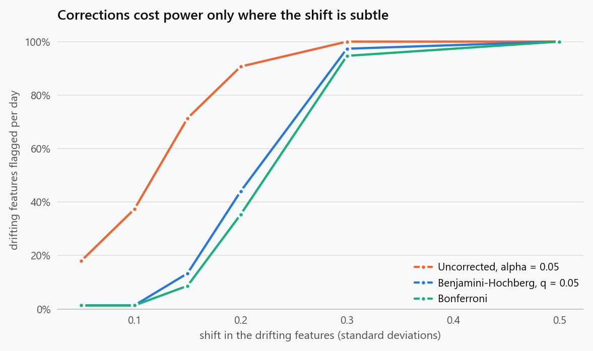
| Shift (sd) | Uncorrected | Bonferroni | Benjamini-Hochberg | Benjamini-Yekutieli |
|---|---|---|---|---|
| 0.05 | 18% | 1% | 1% | 1% |
| 0.10 | 37% | 1% | 1% | 1% |
| 0.15 | 71% | 9% | 13% | 6% |
| 0.20 | 91% | 35% | 44% | 24% |
| 0.30 | 100% | 95% | 97% | 92% |
| 0.50 | 100% | 100% | 100% | 100% |
Below 0.15 standard deviations nothing corrected finds anything on a given day with 500 records, and the uncorrected monitor's apparent power there is bought with a false discovery rate above 80 percent. At 0.3 and above every procedure finds every drifting feature on day one, and the corrections cost nothing. The region where the choice matters is narrow, roughly 0.15 to 0.3 standard deviations, and in that region Benjamini-Hochberg keeps most of the power that Bonferroni gives up. Subtle drift is where the procedures differ, and subtle drift is what a monitor exists to catch early.
Dependence Between Features
Benjamini-Hochberg's guarantee assumes the tests are independent or positively dependent, which covers most monitoring situations. The Benjamini-Yekutieli variant holds under any dependence, at the cost of dividing $q$ by $\sum_{i=1}^{m} 1/i$, about 5.9 for 200 features. The last column of the table shows the price: at a shift of 0.2 it finds 24 percent of the drifting features where Benjamini-Hochberg finds 44 percent. For a monitor that price is rarely worth paying, since input features are overwhelmingly positively dependent.
Correlation does something else to a monitor that no correction addresses. When features share underlying factors, their p-values move together, and the false alerts stop arriving as a steady trickle.
1
2
3
4
5
6
7
8
9
10
11
12
13
14
15
16
17
18
19
20
rng_c = np.random.default_rng(21)
loadings = rng_c.normal(size=(n_features, 10)) * np.sqrt(0.8 / 10)   # 80% shared variance

def correlated_batch(n):
    factors = rng_c.normal(size=(n, 10))
    return factors @ loadings.T + rng_c.normal(scale=np.sqrt(0.2), size=(n, n_features))

independent, correlated = [], []
for _ in range(60):
    p_ind = np.array([stats.ks_2samp(rng_c.normal(size=n_ref), rng_c.normal(size=n_batch)).pvalue
                      for _ in range(n_features)])
    ref, new = correlated_batch(n_ref), correlated_batch(n_batch)
    p_cor = np.array([stats.ks_2samp(ref[:, j], new[:, j]).pvalue for j in range(n_features)])
    independent.append((p_ind < alpha).sum())
    correlated.append((p_cor < alpha).sum())

for name, c in (("independent", independent), ("correlated", correlated)):
    c = np.array(c)
    print(f"{name:<12} mean {c.mean():.1f}, sd {c.std():.1f}, max {c.max()}, "
          f"days over 20: {(c > 20).sum()}, days at 2 or fewer: {(c <= 2).sum()}")
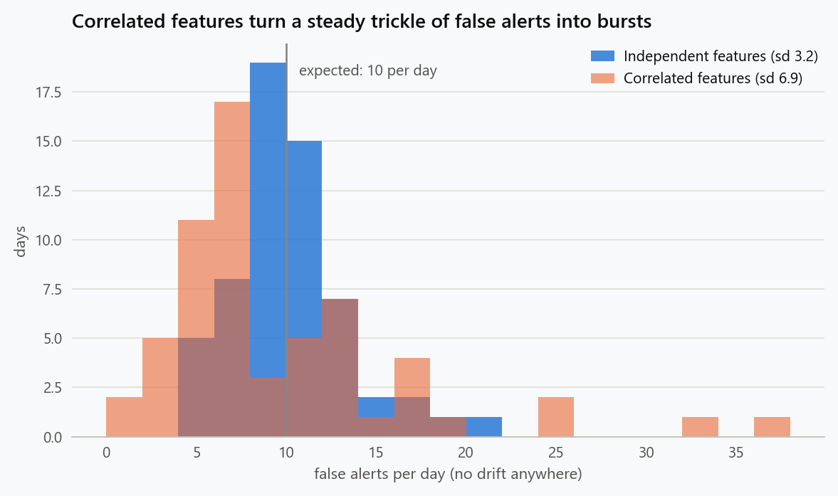
Both monitors average about ten false alerts a day. The independent one has a standard deviation of 3.2, one day above 20 in two months and none with two alerts or fewer. The correlated one has a standard deviation of 6.9, reaches 36, has four days above 20 and four days with two alerts or fewer. Nothing is drifting on any of those days. A burst of alerts on correlated features is what a quiet day looks like when a batch happens to sit a little off-centre on one shared factor, and a monitor that escalates on "many features at once" will escalate on noise.
The constructive response is to treat correlated features as one thing. Cluster the features on their correlation, test each cluster once with a multivariate statistic or on its first principal component, and run the per-feature tests only inside a cluster that fired. Real drift on a shared factor then produces one alert with a list of affected features attached, rather than twenty alerts that all describe the same event.
Time Is the Other Dimension
Correcting across features each day leaves the multiplicity across days untouched. A stable feature gets thirty chances a month to fail a 5 percent test, so it will, and the day-to-day pattern of a false alert is that it fires once and disappears.
Real drift persists. The simplest way to use that is a persistence rule: alert only when a feature has failed the test on several consecutive days.
1
2
3
4
5
6
7
8
9
consecutive = np.zeros(n_features, dtype=int)
tp = fp = 0
for _ in range(n_days):
    p = daily_pvalues(shift)
    consecutive = np.where(p < alpha, consecutive + 1, 0)
    fired = consecutive >= 3
    tp += fired[drifted].sum()
    fp += fired.sum() - fired[drifted].sum()
print(f"3-day persistence: true {tp / n_days:.2f}/day, false {fp / n_days:.2f}/day")
Requiring three consecutive days at the uncorrected level gives 3.67 true alerts per day and no false alerts at all in this run. The expectation is not zero, but it is small: with $d$ days and $m$ stable features the expected number of false alerts per month is about $(d - 2)\, m\, \alpha^3$, which is 0.7 for 200 features, against 293 without the rule. The true-alert rate is below the uncorrected 4.67 because nothing can fire in the first two days and each day's alert needs three rejections in a row. The price is a delay of two days before any drift can be reported, and a slow drift that hovers around the threshold can go unreported for longer. Persistence rules are an informal sequential test. Formal ones, such as CUSUM charts and always-valid p-values, deliver the same protection with an explicit bound on the detection delay, and they are the right tool when the delay matters.
The reference window matters too. A reference that rolls forward with recent data lets slow drift walk in unnoticed, because each day is compared with days that have already drifted. A reference frozen at training time treats every seasonal change as drift. Neither is wrong; each has to be chosen knowing which failures it hides.
Significance Is Not Importance
With enough data every test rejects. A shift of 0.03 standard deviations is operationally nothing for almost any model.
1
2
3
4
for n in (500, 5000, 50000):
    ps = [stats.ks_2samp(rng.normal(size=n), rng.normal(loc=0.03, size=n)).pvalue
          for _ in range(200)]
    print(f"n = {n:>6}: rejected in {np.mean(np.array(ps) < 0.05):.0%} of runs")
At 500 points per batch the shift is invisible, rejected in 6 percent of runs. At 5,000 it is 26 percent, and at 50,000 it is flagged 98 percent of the time. A monitor on a high-volume model will therefore report drift on every feature, every day, once the batches are large enough, and none of the corrections above address that. They are corrections for false positives, and these are true positives that do not matter.
The fix is to require two conditions: the shift is detectable, and it is large enough to care about. The p-value answers the first. An effect size answers the second, and the Wasserstein distance in units of the feature's standard deviation is a convenient one, because it reads directly as "how far the distribution moved".
1
2
3
4
5
rng = np.random.default_rng(5)
for delta in (0.03, 0.2):
    a, b = rng.normal(size=50000), rng.normal(loc=delta, size=50000)
    print(f"shift {delta}: p = {stats.ks_2samp(a, b).pvalue:.1e}, "
          f"Wasserstein = {stats.wasserstein_distance(a, b):.3f} sd")
Both shifts are significant at 50,000 records per side. The trivial one has a Wasserstein distance of 0.018 standard deviations, the meaningful one 0.206. A gate at 0.1 standard deviations, or a population stability index threshold agreed with the model owner, separates them without any reference to the p-value. That turns the p-value into what it should be in a monitor: a filter against noise, not the decision.
Segments Multiply Everything
Monitoring by segment is good practice, since drift often arrives in one region, one device type or one customer tier before it shows in the aggregate. It also multiplies the number of tests. Two hundred features across twenty segments is 4,000 tests a day, and at an uncorrected 5 percent that is 200 false alerts a day before anything has moved.
The corrections above apply unchanged, with $m$ now the full count of feature-segment pairs, and the false discovery rate is the right quantity to control because the number of true discoveries can be large when a segment drifts as a whole. Small segments add a second problem: a segment with 40 records cannot detect anything short of a large shift, so its alerts are both rare and, when they fire, more likely to be noise. Segment tests should be reported with their sample size and pooled up to a coarser segmentation where the size is too small to matter.
Not Every Feature Deserves the Same Alpha
The features are not equally important to the model. A shift in a feature the model ignores is not a model-risk event, and a shift in the feature that carries most of the signal is. Treating them identically wastes the alert budget.
Weighted versions of Benjamini-Hochberg allow the level to be spent unevenly. A practical form is to weight each feature by its permutation importance, normalised to average one, and test $p_j / w_j$ instead of $p_j$. Features the model relies on get a looser threshold, features it barely uses a stricter one, and the false discovery guarantee survives as long as the weights average one.
The complementary move is to add one test that has no multiplicity problem at all: the distribution of the model's own output. If predictions have not shifted, drift in the inputs is a curiosity; if they have, it is an incident whichever input caused it. A two-stage design follows naturally. Test the output every day as a single gate. Run the per-feature tests, corrected, only when the gate opens or on a slower schedule, so that the per-feature results serve as diagnosis rather than as the alarm.
Designing an Alert Budget
Work backwards from what the team can investigate:
- Set the budget. Decide how many drift investigations per week are affordable. That number, not 0.05, is the design constraint.
- Control the false discovery rate across features with Benjamini-Hochberg, choosing $q$ so that the expected false alerts fit the budget.
- Collapse correlated features into clusters and test the cluster, so that one event produces one alert.
- Add persistence across days, or a sequential test if detection delay is critical.
- Gate on effect size so that high-volume batches do not report trivial shifts.
- Weight by feature importance and monitor the output distribution as the single, uncorrected gate.
- Track the monitor's own precision. Log the share of alerts that led to a confirmed issue. If it falls below the target, the monitor has drifted, and it gets tuned like any other model.
With 200 features, Benjamini-Hochberg at $q = 0.05$, a three-day persistence rule and an effect-size gate, the simulated monitor produces well under one false alert a month and still reports a 0.2 standard deviation shift within days. A monitor that fires ten times a day is not vigilant. It is noise with a dashboard, and the arithmetic that makes it so has been known since before the first model was deployed.
The figure generator in the blog-reproducibility repository reproduces this article's figures; run it with --dry-run to print the numbers behind the figures without writing an image.
References
- Benjamini, Y., & Hochberg, Y. (1995). Controlling the false discovery rate: a practical and powerful approach to multiple testing. Journal of the Royal Statistical Society: Series B, 57(1), 289-300.
- Benjamini, Y., & Yekutieli, D. (2001). The control of the false discovery rate in multiple testing under dependency. The Annals of Statistics, 29(4), 1165-1188.
- Holm, S. (1979). A simple sequentially rejective multiple test procedure. Scandinavian Journal of Statistics, 6(2), 65-70.
- Genovese, C. R., Roeder, K., & Wasserman, L. (2006). False discovery control with p-value weighting. Biometrika, 93(3), 509-524.
- Storey, J. D., & Tibshirani, R. (2003). Statistical significance for genomewide studies. Proceedings of the National Academy of Sciences, 100(16), 9440-9445.
- Rabanser, S., Günnemann, S., & Lipton, Z. C. (2019). Failing loudly: an empirical study of methods for detecting dataset shift. Advances in Neural Information Processing Systems, 32.
- Efron, B. (2010). Large-Scale Inference: Empirical Bayes Methods for Estimation, Testing, and Prediction. Cambridge University Press.
Embed interactive plots, widgets, and demos using <figure>, <iframe>, or <div class="interactive-embed"> containers. Ensure each embed includes descriptive captions for accessibility.
How to cite
Use the quick export buttons to save citations for reference managers or copy the formatted text directly.
Diogo Ribeiro (2026). Multiple Comparisons in Model Monitoring: Why the Alerts Never Stop. Faculty of Media Arts and Design, Technical University of Porto. https://diogoribeiro7.github.io/machine-learning/multiple_comparisons_model_monitoring/.


