LoRA Is a Low-Rank Model of the Fine-Tuning Update

LoRA is commonly introduced as a way to fine-tune a large language model without updating all of its parameters. That description is operationally correct, but it misses the mathematical assumption that makes the method interesting.

LoRA does not merely reduce the number of trainable parameters. It constrains the fine-tuning update itself to be low rank.

If a pretrained layer has weight matrix

full fine-tuning learns an unrestricted update

so that

LoRA replaces that unrestricted update by

where

and

The rank therefore satisfies

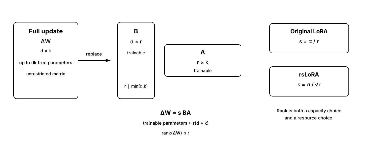
The number of trainable parameters changes from approximately

to

That reduction is important, but it is a consequence of the structural assumption. The deeper claim is that the useful part of the fine-tuning update may lie in a low-dimensional subspace.

Rank is a modelling assumption

Suppose the full fine-tuning update that would be learned without constraints is

Its singular-value decomposition is

with singular values

The best rank-$r$ approximation in Frobenius norm is obtained by truncating the SVD:

By the Eckart–Young theorem,

This equation provides the clearest interpretation of LoRA rank.

If the singular spectrum decays quickly, a small $r$ can represent most of the update energy. If the spectrum is flat, a small-rank adapter necessarily discards a substantial part of the unrestricted update.

LoRA training does not compute the SVD of a previously learned full update. It learns $A$ and $B$ directly. But the approximation argument explains what rank controls.

A rank of 8 is not inherently efficient or sufficient. It is a hypothesis that eight latent update directions are enough for the task.

Small rank can regularize as well as compress

Constraining the update can help even when memory is not the primary concern.

A full $d\times k$ update has many degrees of freedom. A low-rank factorization reduces the accessible parameter space.

The unrestricted update space has dimension approximately

whereas the factorization uses approximately

parameters.

This can act as an implicit regularizer, particularly on small datasets. The adapter cannot move independently in every direction of the full weight space.

But this should not be romanticized. A restrictive low-rank update can also underfit. If performance saturates far below the required target while training remains stable, rank may be one of the constraints worth testing.

The relevant question is empirical:

Does increasing rank improve held-out behaviour enough to justify the extra capacity?

Rank should be tuned against held-out behaviour

A simple rank experiment might compare

For each rank, keep the training data, optimizer family, evaluation prompts and decoding configuration fixed.

Track at least:

• target-task metric,
• regression metrics,
• validation loss,
• trainable parameter count,
• peak GPU memory,
• training throughput,
• adapter size.

The result is a trade-off surface, not a one-dimensional leaderboard.

If rank 16 performs indistinguishably from rank 64 on held-out behaviour, the larger adapter may be unnecessary.

If rank 4 trains faster but systematically misses rare behaviours, the smaller adapter may be too restrictive.

The LoRA scaling factor matters

The original LoRA formulation commonly scales the low-rank update as

where $\alpha$ is often called lora_alpha.

The ratio

controls the magnitude of the adapter contribution relative to the frozen base layer.

This creates an interaction between rank and alpha. Changing $r$ while keeping $\alpha$ fixed changes the scale of the update.

That means a rank sweep is not fully interpretable if the scaling convention changes the effective update magnitude dramatically across ranks.

Rank-stabilized LoRA addresses this by using a scaling proportional to

instead of

The goal is to improve scaling behaviour as rank increases.

In PEFT this is exposed through use_rslora=True.

A configuration may therefore look like:

1
2
3
4
5
6
7
8
9
10
from peft import LoraConfig

peft_config = LoraConfig(
    r=32,
    lora_alpha=32,
    use_rslora=True,
    target_modules="all-linear",
    lora_dropout=0.05,
    task_type="CAUSAL_LM",
)

The important point is not that rsLoRA is universally superior. It is that rank and scaling are coupled design decisions.

Target modules define where the model is allowed to adapt

LoRA does not need to be attached to every linear layer.

A transformer contains several families of projections. Depending on architecture, these may include attention projections such as

1
2
3
4
q_proj
k_proj
v_proj
o_proj

and feed-forward projections such as

1
2
3
4
5
6
7
8
9
10
11
12
13
14
gate_proj
up_proj
down_proj
```.

Adapting only query and value projections produces a much smaller adapter than adapting every linear layer.

A narrow configuration might use

```python
target_modules=[
    "q_proj",
    "v_proj",
]

whereas a broad QLoRA-style configuration often uses

1
2
3
4
5
6
7
8
9
10
11
12
13
14
15
16
17
18
19
20
21
22
23
24
25
26
27
28
29
30
31
32
33
34
35
36
37
38
39
40
41
42
43
44
45
46
47
48
49
50
51
52
target_modules="all-linear"
```.

These are not interchangeable choices.

The target-module set determines which subspaces of the network can change. A model may require only modest attention adaptation for one task and broader feed-forward adaptation for another.

Target-module selection should therefore be treated like architecture selection.

## Parameter count should be reported explicitly

Suppose a model has $L$ adapted matrices, with matrix $j$ having shape

$$
d_j\times k_j.
$$

A LoRA adapter of rank $r_j$ adds approximately

$$
r_j(d_j+k_j)
$$

trainable parameters for that matrix.

Across all adapted layers,

$$
P_{\mathrm{LoRA}}
=
\sum_{j=1}^{L}
r_j(d_j+k_j).
$$

The useful quantity to report is the trainable fraction

$$
\rho
=
\frac{
P_{\mathrm{trainable}}
}{
P_{\mathrm{total}}
}.
$$

Calling a method "parameter efficient" without reporting the trainable parameter count hides an important experimental condition.

In PEFT, inspect it directly:

```python
model.print_trainable_parameters()

or through the wrapped trainer model.

Different layers do not need the same rank

A uniform rank is convenient, but there is no theoretical requirement that every adapted layer needs the same capacity.

PEFT supports layer-specific rank patterns.

For example:

1
2
3
4
5
6
7
8
9
10
11
12
13
14
15
16
from peft import LoraConfig

peft_config = LoraConfig(
    r=8,
    lora_alpha=16,
    target_modules="all-linear",
    rank_pattern={
        "model.layers.0.self_attn.q_proj": 16,
        "model.layers.1.self_attn.q_proj": 16,
    },
    alpha_pattern={
        "model.layers.0.self_attn.q_proj": 32,
        "model.layers.1.self_attn.q_proj": 32,
    },
    task_type="CAUSAL_LM",
)

This is useful when evidence suggests that some layers benefit from more adaptation capacity than others.

But arbitrary per-layer patterns create a large hyperparameter space.

Unless there is a principled reason, uniform configurations are easier to evaluate and reproduce.

LoRA dropout is ordinary regularization

lora_dropout applies dropout on the adapter pathway during training.

It does not affect the frozen base weights directly.

A configuration such as

is a regularization choice, not a default law.

On a large, diverse dataset, dropout may provide little benefit. On a small adaptation dataset, it can reduce overfitting.

The choice should be evaluated against held-out behaviour.

Initialization affects early optimization

In standard LoRA, one factor is typically initialized so that the initial adapter contribution is zero or near zero.

This has an important property:

The adapted model therefore begins close to the original base model.

Several newer initialization strategies attempt to improve optimization by using information from activations or weight structure rather than purely random initialization.

Examples exposed in current PEFT tooling include variants such as PiSSA and LoftQ-related initialization strategies.

These approaches can matter when adaptation budgets are tight, but they introduce another experimental factor. They should not be mixed into a comparison unless the question is specifically about initialization.

QLoRA changes storage precision, not the rank constraint

QLoRA combines LoRA with a quantized frozen base model.

The trainable update remains

The frozen base is represented approximately as

often using 4-bit quantization.

The effective computation becomes approximately

LoRA controls the dimensionality of the update.

Quantization controls the representation cost of the frozen base.

These are orthogonal ideas.

This is why QLoRA should not be described as a different adaptation objective. It is LoRA under a memory-efficient base-model representation.

DoRA decomposes magnitude and direction

DoRA, or Weight-Decomposed Low-Rank Adaptation, modifies the adaptation view by separating the magnitude and direction of pretrained weights.

A weight vector can be written schematically as

where $m$ controls magnitude and $v$ controls direction.

DoRA learns updates in a way that treats these components separately, while still using low-rank adaptation for directional changes.

The intuition is that full fine-tuning can alter both the direction and magnitude of weights, while ordinary LoRA primarily parameterizes an additive update. Explicitly modelling magnitude can narrow part of that gap.

In PEFT this can be enabled through a configuration such as

1
2
3
4
5
6
7
peft_config = LoraConfig(
    r=16,
    lora_alpha=32,
    target_modules="all-linear",
    use_dora=True,
    task_type="CAUSAL_LM",
)

DoRA can improve quality in some regimes, but it also introduces additional computation and state. It belongs in an ablation, not in an unquestioned default stack.

Compare LoRA variants factorially

A useful experiment might vary

scaling

and adaptation type

The resulting design can be treated as

where $Y$ includes behavioural performance and resource metrics.

The point is not to create a giant hyperparameter search.

The point is to avoid attributing an improvement to "LoRA" when several structural changes were made simultaneously.

Adapter merging is an algebraic operation

During inference, a LoRA layer computes

If deployment does not need to preserve the adapter separately, the matrices can be merged:

Then inference becomes

This removes the separate adapter branch from the forward pass.

In PEFT:

1
merged_model = model.merge_and_unload()

Merging changes packaging and sometimes inference efficiency.

It does not create a better model.

The unmerged adapter remains useful when:

• several adapters share one base model,
• adapters need to be switched dynamically,
• storage efficiency matters,
• independent versioning is required.

Multi-adapter serving changes the economics

Suppose there are $m$ clients or tasks.

Full fine-tuning may require storing approximately

parameters for a base model of size $P$.

A shared base with adapters requires approximately

where

This is one of LoRA's strongest operational advantages.

A single base model can support several adapters for:

• different domains,
• different clients,
• different response styles,
• different tools,
• different languages,
• different task families.

The problem then shifts from model storage to adapter routing and lifecycle management.

Which adapter applies to which request? Can two adapters be composed safely? Which version is active? Can an adapter be hot-swapped without disturbing concurrent requests?

These are serving questions, not training questions.

Adapter composition is not automatically additive in behaviour

Because LoRA updates are matrices, it is tempting to combine two adapters as

Algebraically this is straightforward.

Behaviourally it is not guaranteed to be meaningful.

Two adapters may alter overlapping directions in weight space. Their combination can reinforce, cancel or distort behaviours.

Weighted adapter composition should therefore be evaluated as a new model configuration.

It is not safe to infer that if adapter A is good and adapter B is good, then A+B is better.

Low rank can be tested indirectly

The ideal way to know whether the true useful update is low rank would be to compare against a full fine-tuning update and inspect its singular values.

For many large models that is impractical.

A more realistic diagnostic is behavioural saturation.

Train a rank sequence

If the held-out metric stabilizes after a modest rank,

then additional update capacity is not producing measurable benefit under the current dataset and objective.

That does not prove the unrestricted update is mathematically low rank.

It does show that the task does not appear to need more adapter capacity at the resolution of the evaluation.

High rank can hide a data problem

If performance improves every time rank increases, the obvious conclusion is that the adapter needs more capacity.

That may be true.

But it can also indicate:

• noisy labels,
• inconsistent formatting,
• heterogeneous tasks forced into one adapter,
• under-specified prompts,
• poor target-module choices,
• inadequate training duration.

Increasing rank should not become the LLM equivalent of increasing polynomial degree until the training set fits.

Capacity can absorb noise.

The right comparison includes generalization and regression metrics.

LoRA does not remove optimizer-state costs entirely

LoRA dramatically reduces optimizer state because gradients are stored only for trainable adapter parameters.

But activation memory remains.

For long sequences, activation memory can dominate.

Approximate memory therefore includes several terms:

QLoRA reduces $M_{\mathrm{base}}$.

LoRA reduces $M_{\mathrm{adapter}}+M_{\mathrm{optimizer}}$ relative to full fine-tuning.

Gradient checkpointing reduces activation memory at the cost of extra compute.

No single technique removes every memory term.

Trainable-parameter efficiency is not compute efficiency

A model can have very few trainable parameters while still requiring an expensive forward and backward pass through the full base network.

This distinction matters.

LoRA reduces the number of updated weights.

It does not reduce the number of frozen base-model operations needed to produce activations.

Training time therefore does not scale directly with the trainable parameter fraction.

Similarly, a tiny adapter does not make a 70-billion-parameter base model cheap to serve.

Parameter efficiency and system efficiency are related but distinct.

Evaluate LoRA against the right baselines

A meaningful adaptation study should not compare one LoRA configuration only against the unadapted base.

Useful baselines include:

and, when feasible,

Within LoRA, compare at least one smaller and one larger rank.

If QLoRA is used, separate the adaptation question from the quantization question where possible.

Otherwise improvements or regressions can be attributed to the wrong component.

A practical PEFT configuration should be explicit

A readable configuration is better than a mysterious one copied from a notebook.

For example:

1
2
3
4
5
6
7
8
9
10
11
from peft import LoraConfig

peft_config = LoraConfig(
    r=16,
    lora_alpha=32,
    lora_dropout=0.05,
    target_modules="all-linear",
    bias="none",
    task_type="CAUSAL_LM",
    use_rslora=True,
)

The accompanying experiment log should record:

• rank,
• alpha,
• scaling convention,
• dropout,
• target modules,
• initialization,
• base-model revision,
• quantization settings,
• trainable parameter count,
• dataset version,
• training seed.

The adapter file alone is not the experiment.

The adapter should be treated as a statistical model

It is tempting to think of LoRA as an implementation detail because the base model dominates the parameter count.

That is misleading.

The adapter is a fitted object learned from finite data.

It has:

• capacity,
• hyperparameters,
• initialization,
• optimization error,
• sampling variability,
• overfitting risk,
• deployment assumptions.

The same standards used for other statistical models apply.

A rank-16 adapter trained once on one split and selected because it "looks good" is not exempt from model-selection bias merely because it is attached to an LLM.

The most important LoRA question is not how small the adapter is

The most important question is whether the low-rank constraint preserves the behavioural change that matters.

A tiny adapter that fails the target task is not efficient.

A large adapter that reproduces full fine-tuning quality may still be worthwhile if it enables modular serving and shared base weights.

The correct objective is therefore not

alone.

It is closer to

LoRA gives a powerful way to move along that trade-off.

It does not eliminate the need to define it.

References

Dettmers, T., Pagnoni, A., Holtzman, A., & Zettlemoyer, L. (2023). QLoRA: Efficient Finetuning of Quantized LLMs. Advances in Neural Information Processing Systems, 36.

Hu, E. J., Shen, Y., Wallis, P., Allen-Zhu, Z., Li, Y., Wang, S., Wang, L., & Chen, W. (2022). LoRA: Low-Rank Adaptation of Large Language Models. International Conference on Learning Representations.

Hugging Face. PEFT documentation: LoRA. Accessed 20 September 2026.

Liu, S.-Y., Wang, C.-Y., Yin, H., Molchanov, P., Wang, Y.-C. F., Cheng, K.-T., & Chen, M.-H. (2024). DoRA: Weight-Decomposed Low-Rank Adaptation. Proceedings of ICML 2024.

Kalajdzievski, D. (2023). A Rank Stabilization Scaling Factor for Fine-Tuning with LoRA. arXiv:2312.03732.