Topics
The request arrives as a budget line. Labeling another ten thousand examples will cost twenty thousand euros and six weeks. Will the model be better enough to justify it? The usual answers are a shrug and "more data is always better". Neither is an estimate. The learning curve is, and it is cheap to produce from data already in hand.
What the Curve Shows
A learning curve plots error on a fixed test set against the number of training examples. Its shape has two parts. The level it descends toward is the floor: the error the model class would reach with unlimited data, which is the irreducible error of the task plus whatever the model's assumptions cannot capture. The speed of the descent is how much each additional example is worth, and it falls as the training set grows.
For a wide range of models the curve is well described by a power law,
with $a$ the floor, $c$ the rate of approach, and $b$ a scale. Cortes and colleagues proposed the form in 1994; Hestness and colleagues found it holding across deep learning tasks over several orders of magnitude of data. The exponent is typically between 0.3 and 1, and the three parameters are all that is needed to say what more data will buy.
A Simulation With a Known Floor
The task has twelve features, of which five matter, including an interaction and a quadratic term that a linear model cannot represent. Because the true probabilities are known, the Bayes error rate is known, and it is the floor that no model can beat.
1
2
3
4
5
6
7
8
9
10
11
12
13
14
15
16
17
18
19
20
21
22
23
24
25
26
27
28
29
30
31
32
33
34
35
36
37
38
39
40
41
42
43
import numpy as np
from scipy.optimize import curve_fit
from sklearn.ensemble import HistGradientBoostingClassifier
from sklearn.linear_model import LogisticRegression

rng = np.random.default_rng(0)

def make(n, r):
    X = r.normal(size=(n, 12))
    logit = (1.2 * X[:, 0] - 1.0 * X[:, 1] + 0.8 * X[:, 2] + 1.5 * X[:, 0] * X[:, 1]
             + 1.0 * (X[:, 3] ** 2 - 1) - 0.6 * X[:, 4])
    p = 1 / (1 + np.exp(-logit))
    return X, (r.uniform(size=n) < p).astype(int), p

Xte, yte, pte = make(50000, rng)
bayes = np.mean(np.minimum(pte, 1 - pte))
print(f"Bayes error rate = {bayes:.3f}; positive rate {yte.mean():.3f}")

sizes = [250, 500, 1000, 2000, 4000, 8000, 16000, 32000]
Xpool, ypool, _ = make(32000 * 3, rng)     # pool to draw training sets from
models = {
    "logistic": lambda: LogisticRegression(max_iter=2000),
    "boosting": lambda: HistGradientBoostingClassifier(max_iter=300, learning_rate=0.05,
                                                       early_stopping=True, random_state=0),
}
curves = {k: [] for k in models}
train_err = {k: [] for k in models}
sds = {k: [] for k in models}
for n in sizes:
    for name, mk in models.items():
        errs, terrs = [], []
        for rep in range(3):                 # three random training sets per size
            idx = np.random.default_rng(100 * n + rep).choice(len(Xpool), n, replace=False)
            m = mk().fit(Xpool[idx], ypool[idx])
            errs.append(1 - (m.predict(Xte) == yte).mean())
            terrs.append(1 - (m.predict(Xpool[idx]) == ypool[idx]).mean())
        curves[name].append(np.mean(errs))
        sds[name].append(np.std(errs))
        train_err[name].append(np.mean(terrs))
print("\nn        logistic test  (train)   boosting test  (train)   sd over 3 draws (boosting)")
for i, n in enumerate(sizes):
    print(f"{n:<8} {curves['logistic'][i]:.3f}         ({train_err['logistic'][i]:.3f})   "
          f"{curves['boosting'][i]:.3f}          ({train_err['boosting'][i]:.3f})   {sds['boosting'][i]:.3f}")
| Training examples | Logistic test error | Logistic training error | Boosting test error | Boosting training error |
|---|---|---|---|---|
| 250 | 0.326 | 0.297 | 0.296 | 0.127 |
| 500 | 0.317 | 0.289 | 0.266 | 0.065 |
| 1,000 | 0.304 | 0.306 | 0.245 | 0.050 |
| 2,000 | 0.301 | 0.283 | 0.232 | 0.070 |
| 4,000 | 0.300 | 0.297 | 0.224 | 0.105 |
| 8,000 | 0.298 | 0.292 | 0.218 | 0.146 |
| 16,000 | 0.298 | 0.296 | 0.215 | 0.167 |
| 32,000 | 0.298 | 0.296 | 0.211 | 0.182 |
The Bayes error is 0.205. The logistic regression stops improving at about a thousand examples and sits at 0.298 from then on, almost ten points above the floor, because no quantity of data teaches a linear model an interaction. The boosting model is better than the logistic one at every size, by three points at 250 examples, and at 32,000 it is within six tenths of a point of the Bayes rate.
The training error column is the diagnostic. At 250 examples the boosting model's training error is 0.127 against a test error of 0.296: a gap of seventeen points, which is variance, and variance is what more data removes. The logistic model's gap is three points at 250 and zero by a thousand. A model with high error and no gap is not short of data. It is short of capacity or of features, and the budget request should be redirected.
The curve is noisy where it is steep. The standard deviation across the three training draws at 250 examples is 0.025, almost as large as the 0.030 difference between the two models at that size; by 1,000 it is 0.002. A learning curve built from one draw per size can show a model getting worse with more data, and the remedy is to average several draws at each size.
Extrapolating the Curve
The useful question is not what the curve did but what it will do. Fit the power law to the five smallest sizes, up to 4,000 examples, and predict the three that were held out.
1
2
3
4
5
6
7
8
9
10
11
12
13
def power(n, a, b, c):
    return a + b * n ** (-c)

for name in models:
    ns = np.array(sizes[:5], float)
    es = np.array(curves[name][:5])
    (a, b, c), _ = curve_fit(power, ns, es, p0=[es[-1] * 0.9, 1.0, 0.5],
                             bounds=([0, 0, 0.05], [1, 100, 2]), maxfev=20000)
    print(f"\n{name}: fit on n <= 4000 -> asymptote a = {a:.3f}, exponent c = {c:.2f}")
    for n in (8000, 16000, 32000):
        i = sizes.index(n)
        print(f"   predicted error at {n:>6} = {power(n, a, b, c):.3f}   actual {curves[name][i]:.3f}")
    print(f"   predicted at 1,000,000 = {power(1e6, a, b, c):.3f}   (Bayes {bayes:.3f})")
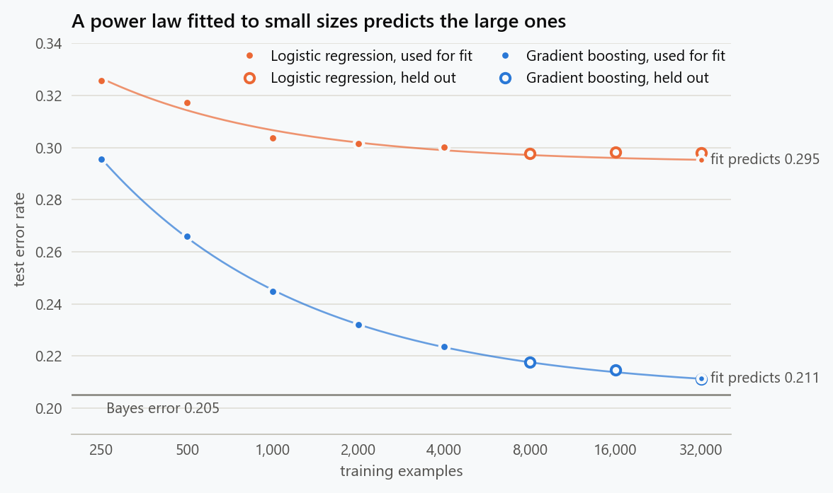
| Model | Fitted floor $a$ | Exponent $c$ | Predicted at 8,000 | Actual | Predicted at 32,000 | Actual |
|---|---|---|---|---|---|---|
| Boosting | 0.206 | 0.60 | 0.218 | 0.218 | 0.211 | 0.211 |
| Logistic | 0.294 | 0.69 | 0.297 | 0.298 | 0.295 | 0.298 |
The fit to the boosting curve, using nothing beyond 4,000 examples, predicts the error at 8,000, 16,000 and 32,000 to within a thousandth, and puts the floor at 0.206 against a true Bayes rate of 0.205. The fit to the logistic curve puts its floor at 0.294, which is the correct message even though the curve had barely moved over the fitted range: this model has finished learning.
Three cautions on the fit. It needs points spanning about a decade of training sizes, and more than four of them, or the three parameters are not identified. It is trustworthy roughly one decade beyond the largest fitted size, which here was the distance from 4,000 to 32,000, and increasingly speculative past that. And it should be fitted to averaged points, because a single noisy value at a small size can move the fitted floor by several points.
Pricing the Next Ten Thousand Labels
The fitted curve makes the budget question arithmetic. From the boosting fit, going from 8,000 to 16,000 examples removes about 0.4 points of error, from 16,000 to 32,000 about 0.3 points, and everything beyond 32,000 combined, all the way to infinite data, at most 0.5 points, because the floor is 0.206 and the curve is at 0.211.
Put a value $V$ on one point of error per year, and a cost $L$ on one label. The doubling from 16,000 to 32,000 costs $16{,}000\,L$ and returns $0.3\,V$ per year. At two euros a label and fifty thousand euros per point, that is 32,000 euros for 15,000 euros a year: a two-year payback, and the doubling after it costs twice as much for less. At some doubling the curve tells the team to stop buying labels.
What it does not tell them is that the model cannot improve. The floor is a property of the model class and the features, and both can be changed. A feature that captures what the model currently cannot moves $a$ down, which no amount of data does. The learning curve separates the two kinds of investment: it prices data against the current floor, and it tells you when the floor is the constraint.
Label Noise Moves the Curve, Not Always the Floor
Training labels are rarely clean, and it is natural to expect noise to raise the floor. Flip ten percent of the training labels at random and rerun the boosting curve, evaluating against the clean test labels.
1
2
3
4
5
6
7
8
9
10
11
12
13
14
15
16
17
flip = np.random.default_rng(7).uniform(size=len(ypool)) < 0.10
ynoisy = np.where(flip, 1 - ypool, ypool)
noisy_curve = []
for n in sizes:
    errs = []
    for rep in range(3):
        idx = np.random.default_rng(100 * n + rep).choice(len(Xpool), n, replace=False)
        m = HistGradientBoostingClassifier(max_iter=300, learning_rate=0.05,
                                           early_stopping=True, random_state=0).fit(Xpool[idx], ynoisy[idx])
        errs.append(1 - (m.predict(Xte) == yte).mean())
    noisy_curve.append(np.mean(errs))
print("10% of training labels flipped, error on clean test labels:")
print("  " + ", ".join(f"{n}: {e:.3f}" for n, e in zip(sizes, noisy_curve)))
(a, b, c), _ = curve_fit(power, np.array(sizes[:5], float), np.array(noisy_curve[:5]),
                         p0=[0.2, 1, 0.5], bounds=([0, 0, 0.05], [1, 100, 2]), maxfev=20000)
print(f"fitted floor {a:.3f}; if the test labels were also 10% noisy the floor would read "
      f"{0.1 + 0.8 * bayes:.3f}")
| Training examples | Clean labels | 10% flipped labels |
|---|---|---|
| 250 | 0.296 | 0.336 |
| 1,000 | 0.245 | 0.267 |
| 4,000 | 0.224 | 0.231 |
| 32,000 | 0.211 | 0.214 |
The noisy curve is shifted to the right, not up: it needs roughly twice the data to reach the same error, and its fitted floor is 0.210, within a hair of the clean one. Symmetric label noise does not change which class is more probable at any point, so the Bayes decision is unchanged and enough data still finds it. What the noise costs is data, and the curve says how much.
The floor moves when the test labels are noisy. With ten percent of test labels flipped, the best possible measured error is not 0.205 but $0.1 + 0.8 \times 0.205 = 0.264$, and no training set of any size brings the curve below it. A team that sees a curve flattening at 0.26 and concludes that the task is hard, or that the model is at capacity, is reading noise in the evaluation. Test labels should be cleaned before the floor is believed, and cleaning them is usually cheaper than cleaning the training set, because there are fewer of them. Noise that is not symmetric, such as one class being mislabeled more often than the other, or mislabeling that depends on the features, does bias the floor, and it is a different problem from the one the curve diagnoses.
When the Curve Misleads
The wrong distribution. The curve measures error on the test distribution. More data from a different distribution flattens the curve without lowering the test error, and a curve that has stalled on data from one source may drop sharply with a little data from the right one.
Rare classes. A curve against total examples hides the count that matters. If the minority class is two percent of the data, a training set of 10,000 has 200 examples of it, and the descent is governed by that number.
Fixed hyperparameters. A model tuned at 1,000 examples is usually over-regularised at 100,000. A curve built with the small-data settings flattens early because the model is not allowed to use the data. Hyperparameters should be retuned at each size, or the curve reports the limits of a configuration rather than of the model class.
Non-stationary data. When the data drift, older examples describe a process that no longer exists, and the curve against "months of history" can turn upward. The horizontal axis is then not the quantity of data but its age.
Regime changes. Deep models sometimes show a plateau followed by a second descent as capacity becomes usable. A power law fitted to the plateau predicts nothing about the descent, and the remedy is the same as always: fit to points that span a decade, and distrust extrapolations far beyond them.
What to Do
- Build the curve with at least five training sizes spanning a decade, three or more random draws at each, and one fixed test set.
- Fit $a + b\,n^{-c}$ to the averaged points and read the floor and the exponent.
- Read the train-test gap. A large gap says data will help; a small gap with high error says the model or the features are the limit.
- Price the next doubling from the fitted curve against the cost of labels, and stop when the return falls below the cost.
- Compare the floor with what is achievable: a stronger model class, inter-annotator agreement, or a known noise level.
- Clean the test labels first, since a noisy evaluation raises the apparent floor and no training data lowers it.
- Retune at each size so that the curve describes the model class, not one configuration of it.
The figure generator in the blog-reproducibility repository reproduces this article's figure; run it with --dry-run to print the numbers behind the figure without writing an image.
References
- Cortes, C., Jackel, L. D., Solla, S. A., Vapnik, V., & Denker, J. S. (1994). Learning curves: asymptotic values and rate of convergence. Advances in Neural Information Processing Systems, 6.
- Hestness, J., Narang, S., Ardalani, N., Diamos, G., Jun, H., Kianinejad, H., Patwary, M. M. A., Yang, Y., & Zhou, Y. (2017). Deep learning scaling is predictable, empirically. arXiv:1712.00409.
- Viering, T., & Loog, M. (2023). The shape of learning curves: a review. IEEE Transactions on Pattern Analysis and Machine Intelligence, 45(6), 7799-7819.
- Figueroa, R. L., Zeng-Treitler, Q., Kandula, S., & Ngo, L. H. (2012). Predicting sample size required for classification performance. BMC Medical Informatics and Decision Making, 12, 8.
- Kaplan, J., McCandlish, S., Henighan, T., Brown, T. B., Chess, B., Child, R., Gray, S., Radford, A., Wu, J., & Amodei, D. (2020). Scaling laws for neural language models. arXiv:2001.08361.
- Domingos, P. (2012). A few useful things to know about machine learning. Communications of the ACM, 55(10), 78-87.
Embed interactive plots, widgets, and demos using <figure>, <iframe>, or <div class="interactive-embed"> containers. Ensure each embed includes descriptive captions for accessibility.
How to cite
Use the quick export buttons to save citations for reference managers or copy the formatted text directly.
Diogo Ribeiro (2026). Learning Curves: Deciding Whether More Data Will Help. Faculty of Media Arts and Design, Technical University of Porto. https://diogoribeiro7.github.io/machine-learning/learning_curves_more_data/.