Topics
Monte Carlo simulations have become a cornerstone of modern quantitative economics, particularly in macroeconomic forecasting, policy stress testing, and uncertainty quantification. By using random sampling to estimate the outcomes of complex systems, these simulations allow economists to probe a range of possible futures—critical for decisions under uncertainty.
This article explores the core mechanics of Monte Carlo methods and illustrates how they're used to simulate stochastic dynamics in macroeconomic models.
🧠 Why Use Monte Carlo in Macroeconomics?
Macroeconomic models are inherently uncertain. Assumptions about technology, policy, and preferences may not hold over time. Monte Carlo simulations help by:
- Capturing stochasticity in model parameters and exogenous shocks
- Quantifying policy risk by simulating outcomes under different interest rate rules or fiscal regimes
- Estimating forecast bands, not just point predictions
- Testing model robustness under worst-case scenarios or rare events
Traditional deterministic simulations offer single trajectories. Monte Carlo offers distributions—essential in policy environments where confidence levels matter.
📐 The Convergence Rate, and Why It Matters
The method rests on the law of large numbers. To estimate $\theta = E[g(X)]$, draw $N$ independent samples and average:
That $\sqrt{N}$ is the defining property of the method, and it cuts both ways. Halving the standard error requires quadrupling the sample, so brute force gets expensive fast: three-decimal precision needs roughly a million draws.
The compensating advantage is that the rate does not depend on dimension. Deterministic quadrature degrades exponentially as dimensions increase, which makes Monte Carlo the only practical option for the high-dimensional integrals that macroeconomic models with many state variables and shocks produce.
Because the error is statistical, it can be reported. Any simulation result quoted without a Monte Carlo standard error is hiding how much of the last digit is noise.
🛠️ Example: Simulating GDP under Random Shocks
Below is a simplified Python example simulating GDP growth over 10 years under stochastic productivity and interest rate shocks:
1
2
3
4
5
6
7
8
9
10
11
12
13
14
15
16
17
18
19
20
import numpy as np
import matplotlib.pyplot as plt

np.random.seed(42)
n_simulations = 1000
years = 10
gdp_initial = 100
gdp_paths = np.zeros((n_simulations, years))
gdp_paths[:, 0] = gdp_initial

for t in range(1, years):
    productivity_shock = np.random.normal(0.02, 0.01, size=n_simulations)
    interest_rate_shock = np.random.normal(-0.01, 0.005, size=n_simulations)
    gdp_paths[:, t] = gdp_paths[:, t-1] * (1 + productivity_shock + interest_rate_shock)

plt.plot(range(years), gdp_paths.T, alpha=0.05, color='gray')
plt.title("Simulated GDP Paths (Monte Carlo)")
plt.xlabel("Year")
plt.ylabel("GDP")
plt.show()
This simple example reveals how even small, random shocks compound significantly over time, yielding a wide range of economic futures.
Summarising the fan is usually more useful than plotting every path:
1
2
3
4
5
6
7
percentiles = np.percentile(gdp_paths, [5, 25, 50, 75, 95], axis=0)
final = gdp_paths[:, -1]

print(f"median final GDP : {np.median(final):.1f}")
print(f"90% interval     : {np.percentile(final, 5):.1f} to {np.percentile(final, 95):.1f}")
print(f"P(GDP < 100)     : {(final < 100).mean():.3f}")
print(f"MC standard error: {final.std(ddof=1) / np.sqrt(n_simulations):.3f}")
The last line is the discipline worth adopting: with 1,000 draws the estimate of the mean carries visible sampling error of its own, and quoting the median to one decimal without it would overstate the precision.
⚠️ Where the Simple Version Misleads
The example above makes three assumptions that rarely hold, and each has a standard fix.
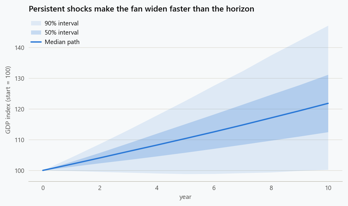
Shocks are independent across time. Real macroeconomic shocks are persistent: a bad productivity year raises the odds of another. Modelling the shock as an AR(1) process, $\varepsilon_t = \rho \varepsilon_{t-1} + \eta_t$, widens the fan considerably, because persistence lets deviations accumulate rather than cancel.
Shocks are independent of each other. Productivity and interest rates are related through policy reaction functions. Drawing them independently understates joint tail events, which are precisely what stress testing exists to find. Correlated draws via a Cholesky factor of the covariance matrix are the minimum correction.
Shocks are normal. Normality assigns negligible probability to the crises that dominate policy discussions. Fat-tailed alternatives such as Student-$t$ innovations, or regime-switching between calm and turbulent states, produce far more realistic extremes.
1
2
3
4
5
6
7
8
9
10
11
12
13
14
15
rng = np.random.default_rng(42)
rho = 0.7                                   # shock persistence
cov = np.array([[0.010**2, -0.3 * 0.010 * 0.005],
                [-0.3 * 0.010 * 0.005, 0.005**2]])
L = np.linalg.cholesky(cov)

eps = np.zeros((n_simulations, 2))
paths = np.full((n_simulations, years), float(gdp_initial))
for t in range(1, years):
    innov = rng.standard_t(df=5, size=(n_simulations, 2)) @ L.T
    eps = rho * eps + innov                 # persistent, correlated, fat-tailed
    growth = 0.02 + eps[:, 0] - 0.01 + eps[:, 1]
    paths[:, t] = paths[:, t-1] * (1 + growth)

print(f"P(GDP < 100), richer model: {(paths[:, -1] < 100).mean():.3f}")
The downside probability under this specification is materially higher than under independent normal shocks, and the gap is the whole point of running the comparison.
🎲 A Note on Randomness and Reproducibility
Seeding matters for more than tidiness. Comparing two policy scenarios under different random draws confounds the policy effect with sampling noise; using common random numbers across scenarios removes that noise and sharply reduces the sample size needed to detect a difference.
Prefer a modern generator object such as np.random.default_rng(seed) over the legacy global np.random.seed, since the global state is easily disturbed by library code elsewhere in a pipeline.
Variance reduction is worth knowing about when budgets bind. Antithetic variates pair each draw with its mirror image, control variates exploit a correlated quantity with known expectation, and importance sampling reweights draws toward the region that matters, which is the standard approach when estimating rare-event probabilities that plain sampling would almost never visit.
🚀 The Road Ahead
Monte Carlo simulations are now central to data-driven economic governance, providing critical insight into both routine fluctuations and rare, high-impact scenarios. As real-time data streams, Bayesian updating, and probabilistic programming advance, the role of these simulations will only expand.
They don't just offer a tool for economists—they represent a mindset: model uncertainty, simulate widely, and prepare for variability.
The caveat that keeps that mindset honest is that a simulation inherits every assumption of the model generating it. A tight fan chart reflects confidence in the specification, not knowledge about the world, and the distributions that matter most in a crisis are exactly the ones estimated from the fewest historical observations.
The figure generator in the blog-reproducibility repository reproduces this article's figure; run it with --dry-run to print the numbers behind the figure without writing an image.
References
- Robert, C. P., & Casella, G. (2004). Monte Carlo Statistical Methods (2nd ed.). Springer.
- Glasserman, P. (2003). Monte Carlo Methods in Financial Engineering. Springer.
- Judd, K. L. (1998). Numerical Methods in Economics. MIT Press.
- Fernández-Villaverde, J., Rubio-Ramírez, J. F., & Schorfheide, F. (2016). Solution and estimation methods for DSGE models. In Handbook of Macroeconomics (Vol. 2). Elsevier.
Embed interactive plots, widgets, and demos using <figure>, <iframe>, or <div class="interactive-embed"> containers. Ensure each embed includes descriptive captions for accessibility.
How to cite
Use the quick export buttons to save citations for reference managers or copy the formatted text directly.
Diogo Ribeiro (2025). Monte Carlo Simulations in Macroeconomic Modeling. Faculty of Media Arts and Design, Technical University of Porto. https://diogoribeiro7.github.io/economics/monte_carlo_simulations_macroeconomic_modeling/.