Topics
A backtest can split its data in perfect chronological order and still use information from the future.
Suppose its first row describes January to March. The analyst treats the row as historical by the end of March. But the value was first published in April, revised in May, and revised again in June. A file downloaded later may contain one of those later estimates beside the original quarter label.
The label describes when economic activity occurred. It does not establish when the estimate became available.
Those are the two dates in the title. An operational system may need further timestamps for retrieval and processing, but separating the economic reference period from information availability is the first step.
One quarter, three public estimates
Consider the first three BEA releases of US real GDP growth for the first quarter of 2025:
| Release | Published at 8:30 a.m. EDT | Growth reported for 2025 Q1 |
|---|---|---|
| Advance estimate | 30 April 2025 | −0.3% |
| Second estimate | 29 May 2025 | −0.2% |
| Third estimate | 26 June 2025 | −0.5% |
All three refer to the same quarter. The rates are seasonally adjusted changes from the previous quarter, expressed at an annual rate. These are archived releases, not a claim about the value in today's database. The third estimate is not necessarily the last revision the quarter will ever receive.
The small CSV used here preserves the reported value, release name, reference period, units, timestamp, and source URL. I transcribed these three rows from the linked releases and checked them on 18 September 2026. All three release times convert to 12:30 UTC, because the stated US time was daylight time.
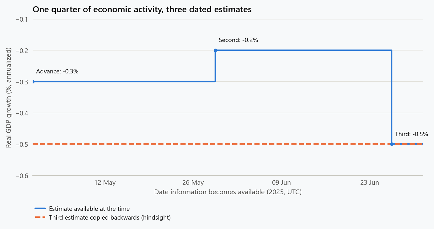
Original timeline from the three archived BEA releases. The horizontal axis tracks information availability; every plotted estimate concerns the same economic quarter. The line stops on 1 July and makes no statement about subsequent releases.
The changes are not three new observations of three successive quarters. They are three versions, or vintages, of an estimate for one quarter.
Make the error visible with a simple decision
Imagine a rule that raises a review flag when the available Q1 growth estimate is below −0.4%. The threshold is arbitrary and fixed for this illustration. It is not an investment strategy or a threshold selected for good performance.
Evaluate the rule at noon UTC on three dates:
| Decision date | Q1 estimate available then | Flag using available data | Flag using the third estimate throughout |
|---|---|---|---|
| 1 May 2025 | −0.3% | No | Yes |
| 1 June 2025 | −0.2% | No | Yes |
| 1 July 2025 | −0.5% | Yes | Yes |
The rule has not changed. Its inputs have. Copying June's release backwards changes the first two decisions using information that did not yet exist in the public record.
Before the advance release, this particular official Q1 estimate is unavailable. The correct value in this example is missing, not zero and not −0.5%. An analyst could have a private forecast or another indicator available earlier, but that would be a different variable with its own provenance.
Nothing in this table proves that the contaminated rule would earn more money or forecast better. Revisions can alter results in either direction. The table establishes a more basic failure: the simulated decisions do not reproduce the specified historical information set.
Select a value by availability
For a particular series and reference period, an as-of lookup selects the most recent release whose usable time is no later than the decision cutoff.
If releases have values $x_1,\ldots,x_k$ and availability times $a_1,\ldots,a_k$, then at cutoff $t$ we use
If no release is eligible, the value is unavailable. That is an information state the rest of the analysis must handle explicitly.
Here is a complete implementation for the supplied CSV, run from the repository root. The file deliberately contains just one series and one reference period:
1
2
3
4
5
6
7
8
9
10
11
12
13
14
15
16
17
18
19
20
21
22
23
import csv
from datetime import datetime
from pathlib import Path

path = Path("assets/data/gdp_q1_2025_release_vintages.csv")
with path.open(encoding="utf-8", newline="") as handle:
    releases = list(csv.DictReader(handle))

for row in releases:
    row["released_at"] = datetime.fromisoformat(row["released_at"])
    row["value"] = float(row["value"])

def as_of(cutoff):
    eligible = [r for r in releases if r["released_at"] <= cutoff]
    if not eligible:
        return None
    return max(eligible, key=lambda r: r["released_at"])["value"]

for day in ("2025-04-29", "2025-05-01", "2025-06-01", "2025-07-01"):
    cutoff = datetime.fromisoformat(day + "T12:00:00+00:00")
    value = as_of(cutoff)
    flag = None if value is None else value < -0.4
    print(day, value, flag)
The output is:
1
2
3
4
2025-04-29 None None
2025-05-01 -0.3 False
2025-06-01 -0.2 False
2025-07-01 -0.5 True
For a larger dataset, apply the selection separately to each series and reference period. Taking the latest timestamp across the whole table would select a release for whichever variable happened to update last.
This example assumes a release becomes usable at its public timestamp. At exactly 12:30 UTC on 30 April, its lookup changes from unavailable to −0.3%. A real system may need to wait for a download, validation, and feature calculation. Its usable timestamp should reflect that process. A date-only table cannot answer whether a value was available for a decision made before that day's release.
Preserve the history before joining tables
A convenient wide table puts one observation per quarter in each row. That shape is useful for modelling, but it hides revisions if there is only one value per cell.
Keep an underlying release table before constructing the modelling view:
| Field | Why it matters |
|---|---|
| Series and reference period | Identify which economic quantity the value describes |
| Value and units | Distinguish levels, changes, rates, and scaling |
| Release or vintage identifier | Preserve successive versions |
| Public release timestamp | Establish the earliest public availability |
| Retrieval and usable timestamps | Represent what the actual system could access |
| Source and transformation version | Make the resulting feature traceable |
For sources where only a vintage date is available, retain that limitation instead of manufacturing an intraday timestamp.
The St. Louis Fed's ALFRED infrastructure exists to retrieve historical information sets. Its documentation distinguishes today's view of past observations from values known during a specified historical real-time period. In the FRED API, realtime_start and realtime_end control that period; their defaults refer to today. St. Louis Fed documentation.
A request with observation_end set to an old date does a different job: it limits the economic periods returned. It does not, by itself, say which vintage of those periods to use. The distinction should be reflected in the query and preserved in the downloaded data. Observation endpoint parameters.
The financial-data version uses the same logic
Suppose a hypothetical company reports results for the year ending 31 December on 20 February. A feature labelled with the year-end date becomes available only when the relevant information is released. If the value is subsequently restated, the original and restated versions need distinct availability records.
That example requires no assumption about a particular company's reporting calendar. It exposes the same data-model requirement as GDP: a fiscal period is not a publication timestamp.
Financial joins also need a declared decision clock. Information released after a market close cannot enter a decision defined as occurring at that close. A later vendor correction may be appropriate for reconstructing what happened, but an execution simulation still needs the quotes, timing, and access assumptions relevant to its decisions.
The appropriate question is specific: which version of this input could this process have used at this cutoff? A chronological train/test split does not answer it if the input values were already overwritten with later versions.
Units and transformations can introduce another mistake
The GDP numbers above are annualized rates. They are not year-over-year changes, and −0.3% annualized does not mean output fell by 0.3% between the two quarters.
For a quarterly growth rate $q$, annualization uses $(1+q)^4-1$. Inverting that expression, −0.3% annualized corresponds to approximately
for the quarter itself. The annualized figure expresses a rate on a common scale; it is not a forecast that the same growth will persist for a year.
The move from −0.2% to −0.5% is a downward revision of 0.3 percentage points in the annualized rate. Keeping the units attached prevents a revision, a quarterly change, and an annualized rate from being treated as interchangeable quantities.
Even after selecting the correct vintages, feature construction must respect the cutoff. For example, a normalisation mean fitted on the entire historical file can include future observations. The availability rule applies to every input used to construct a feature, including fitted transformation parameters.
Revised data still answer useful questions
Revised estimates can be the appropriate input to a retrospective description of economic activity. A forecast can also be evaluated against a declared later-vintage target. Neither choice is inherently an error.
The distinction is between information used to make a historical decision and information used later to judge it. We can evaluate a forecast against a later estimate without pretending that estimate was available as a predictor when the forecast was issued. Training labels require their own availability rule as well: a model fitted in May cannot learn from outcomes first published in June.
A reproducible analysis should state the decision cutoff, the feature vintage policy, and the evaluation target's vintage. If historical vintages are unavailable, that limits the claim: the result describes an analysis of the retrieved data, rather than a fully reconstructed historical decision process.
The figure generator reproduces the release timeline and decision table from the sourced CSV. Three rows are enough to expose the problem. A larger backtest needs to preserve the same information history for every input on which its conclusions depend.
Embed interactive plots, widgets, and demos using <figure>, <iframe>, or <div class="interactive-embed"> containers. Ensure each embed includes descriptive captions for accessibility.
How to cite
Use the quick export buttons to save citations for reference managers or copy the formatted text directly.
Diogo Ribeiro (2026). Economic Data Have Two Dates. Faculty of Media Arts and Design, Technical University of Porto. https://diogoribeiro7.github.io/economics/economic_data_have_two_dates/.