Statistics and Machine Learning: Where the Boundary Actually Lies

The distinction between statistics and machine learning is often explained badly.

One version says that statistics is about inference while machine learning is about prediction. Another says that machine learning is simply statistics performed on larger data sets. A third treats anything with a probability distribution as statistics and anything implemented with an optimizer as machine learning.

None of those boundaries survives contact with actual practice.

Statisticians build predictive models. Machine-learning researchers study uncertainty, identifiability, generalization and causal questions. Linear regression can be taught as a statistical model, an optimization problem or a supervised-learning algorithm without changing the fitted coefficients.

The useful distinction is therefore not a list of algorithms. It is the structure of the problem being solved:

The same mathematical model can behave very differently depending on those choices.

Prediction and inference are different targets

Suppose

A predictive problem asks for a function $\hat f$ that performs well on future observations. A common target is expected prediction loss,

Because the population risk $R(f)$ is unknown, machine-learning procedures usually minimize an empirical or regularized approximation,

An inferential problem can use the same data but ask something different. In the linear model

we might want a confidence interval for one component of $\beta$, a test of a scientific hypothesis, or an estimate of a causal effect under additional identification assumptions. Good prediction does not make those quantities identified. Conversely, a model can estimate a scientifically meaningful parameter well without being the best predictive model available.

This difference in target is more important than the label attached to the method.

Linear regression shows how the two traditions overlap

Ordinary least squares minimizes

That is an optimization problem and therefore fits naturally into supervised learning. Under a Gaussian error model,

the same coefficient estimates are also maximum-likelihood estimates. The probabilistic model then supplies more structure: likelihood-based uncertainty, model diagnostics and a precise statement of the assumptions under which finite-sample inference is derived. The prediction problem does not require every one of those assumptions. If the only goal is out-of-sample squared-error performance, cross-validation can compare predictive procedures without asserting that the errors are exactly Gaussian.

The inferential problem is different. Standard errors, confidence intervals and coefficient interpretations depend on the sampling model and on which assumptions are being used. The algorithm is the same. The claim being made is not.

Regularization makes the loss function explicit

Ridge regression solves

Lasso replaces the quadratic penalty with an $L_1$ penalty,

The important point is not that these are "machine-learning versions" of regression. Both are statistical estimators. Their behavior follows from a deliberate bias-variance trade-off.

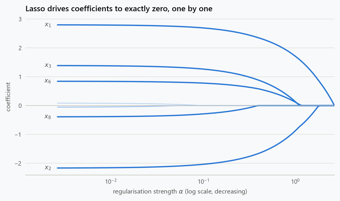
Ridge shrinks unstable coefficients and can improve prediction when predictors are correlated or $p$ is large. Lasso can set coefficients exactly to zero and therefore combines shrinkage with variable selection. But a selected lasso model does not automatically inherit ordinary least-squares inference as if the selected variables had been fixed in advance. Prediction, selection and post-selection inference are distinct problems.

Trees are not statistical because they use Gini impurity

Decision trees are sometimes described as statistical methods because split criteria use quantities such as entropy or Gini impurity. That is not a useful distinction. For a binary node with class proportion $p$, Gini impurity is

and entropy is

A tree searches candidate partitions and chooses splits that reduce an impurity or loss criterion. The difficult statistical question is what happens after repeatedly searching the data for those splits. A deep tree has low training error but high variance. Pruning, minimum leaf sizes and other constraints regularize the search.

Random forests attack the variance problem differently. Each tree is fit to a bootstrap sample and each split considers only a random subset of predictors. Averaging many decorrelated trees can reduce prediction variance substantially.

None of this depends on drawing a boundary between "statistics" and "machine learning." It is an estimation problem involving adaptive search, regularization and out-of-sample validation.

Support vector machines are not probabilistic models by default

A support vector machine is another useful counterexample to loose terminology. For binary labels $y_i\in{-1,+1}$, a soft-margin linear SVM can be written as

The second term is the hinge loss. The first controls the size of $w$, which determines the geometric margin. This is a convex optimization problem arising from statistical learning theory. It is not, in its standard form, a probability model for $P(Y=1\mid X=x)$. The kernel construction changes the representation by replacing inner products with

so that a linear separator in the feature space can represent nonlinear boundaries in the original variables. Calling the kernel trick a "statistical technique" adds little. It is a mathematical device that becomes part of a statistical learning procedure when used to estimate a decision function from data.

Probability models are only one part of machine learning

Other methods start explicitly from probability distributions. Logistic regression models

A Gaussian process places a prior distribution over functions. Hidden Markov models specify a latent-state stochastic process and an observation model. Bayesian neural networks place probability distributions over parameters or functions.

These methods live comfortably in both statistical and machine-learning literatures.

But it is important not to reverse the statement. Hidden Markov models are not inherently Bayesian, and an algorithm does not become Bayesian merely because it uses probabilities. Bayesian inference requires a prior together with a likelihood and a posterior update.

Validation exposes a genuine difference in emphasis

One of the clearest historical differences is the role assigned to prediction on unseen data.

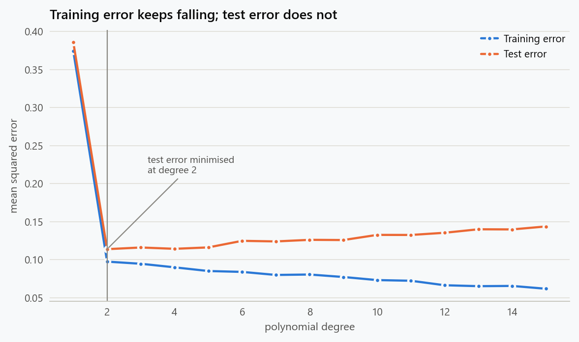
For a predictive system, the relevant quantity is usually generalization error. A training metric is optimistic because the same observations influenced the fitted model. Validation therefore uses held-out data, cross-validation, time-respecting backtests or an external test set.

For a statistical model used primarily for inference, validation also includes model checking: residual structure, calibration, specification, sensitivity to assumptions and whether the sampling design supports the intended interpretation. These are not competing philosophies. A serious analysis often needs both.

A clinical risk model can require good calibration and discrimination on new patients while also needing uncertainty estimates. A causal model may need predictive components internally while the final target is a treatment effect. A forecasting system can have an excellent likelihood fit and still fail operationally out of sample.

Breiman's "two cultures" is a useful historical description, not a law

Leo Breiman described a tension between a data-modeling culture, which starts from an explicit stochastic model, and an algorithmic-modeling culture, which treats the mechanism as largely unknown and emphasizes prediction. That distinction remains useful because it describes different habits of thought. It should not be turned into a rigid taxonomy.

Modern statistical learning contains both cultures. Generalized additive models, boosting, Bayesian hierarchical models, random forests, Gaussian processes and neural networks can all be studied with statistical questions about risk, uncertainty and generalization. The better question is therefore not

Is this statistics or machine learning?

It is

What quantity is being estimated, what assumptions connect the data to that quantity, what loss is being optimized, and how will the claim be validated?

That question survives changes in software, terminology and fashion.

The figure generator in the blog-reproducibility repository reproduces this article's figures; run it with --dry-run to print the numbers behind the figures without writing an image.

References

• Breiman, L. (2001). Statistical modeling: The two cultures. Statistical Science, 16(3), 199–231. https://doi.org/10.1214/ss/1009213726
• Breiman, L. (2001). Random forests. Machine Learning, 45, 5–32. https://doi.org/10.1023/A:1010933404324
• Cortes, C., & Vapnik, V. (1995). Support-vector networks. Machine Learning, 20, 273–297. https://doi.org/10.1007/BF00994018
• Hastie, T., Tibshirani, R., & Friedman, J. (2009). The Elements of Statistical Learning (2nd ed.). Springer.
• Tibshirani, R. (1996). Regression shrinkage and selection via the lasso. Journal of the Royal Statistical Society: Series B, 58(1), 267–288. https://doi.org/10.1111/j.2517-6161.1996.tb02080.x