Topics
The challenger is not supposed to be better. It is cheaper to run, or simpler to maintain, or uses three features instead of thirty, and the only thing it has to show is that it is not worse. The team scores both models on the same test set, runs a paired t-test on the per-item losses, gets a p-value of 0.4, and writes that there is no significant difference and the models are equivalent. The challenger ships.
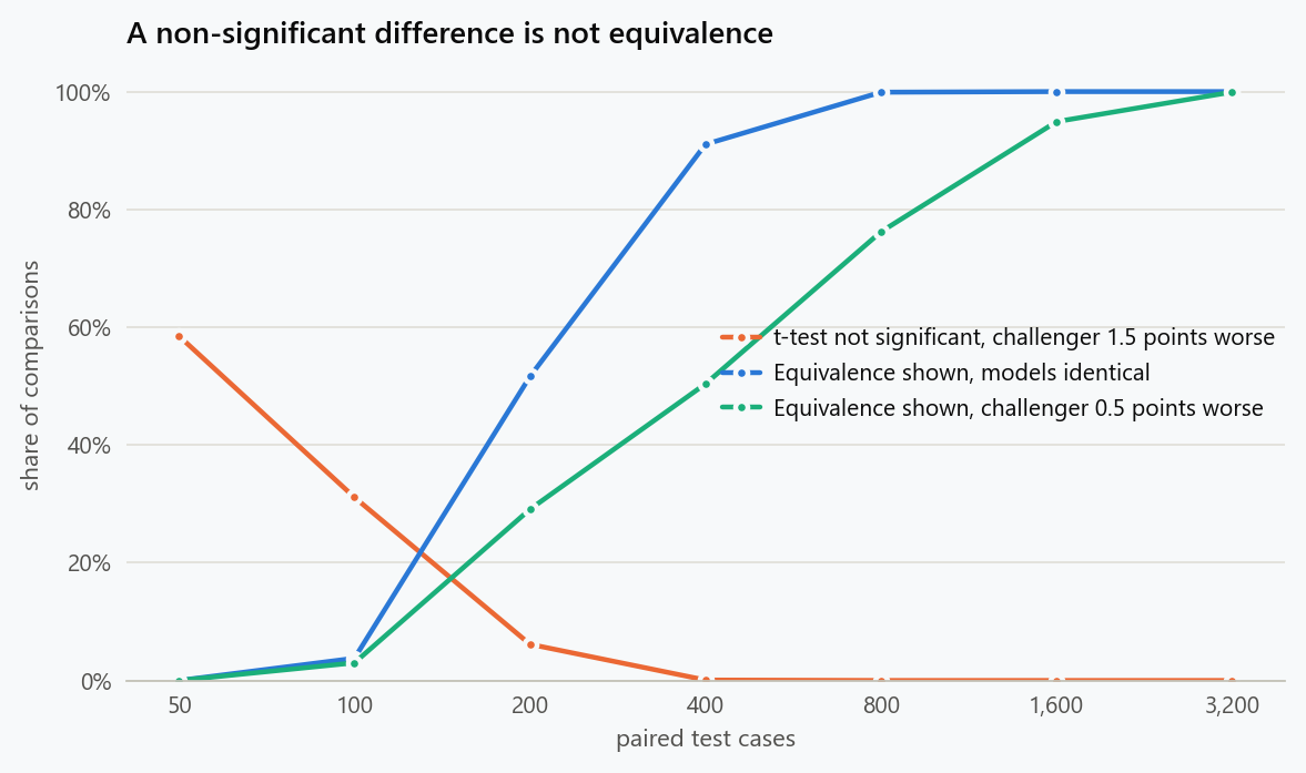
They have shown nothing. A non-significant test says the data are compatible with no difference. The data are also compatible with a difference large enough to matter, and with fifty test cases they usually are. A challenger that is truly 1.5 points worse produces a non-significant result 59 percent of the time at that size.
Absence of Evidence
The two-sided test puts "no difference" in the null hypothesis. Rejecting it demonstrates a difference; failing to reject it demonstrates that the test lacked either a difference or the power to find one, and does not say which. To demonstrate "no worse", the claim has to move into the alternative hypothesis, where evidence can support it.
That requires a margin: the largest deterioration $\delta$ that would still count as no worse. The claim then has two forms.
Non-inferiority. The null is that the challenger is worse by at least $\delta$; the alternative is that it is not. One one-sided test.
Equivalence. The null is that the difference lies outside $(-\delta, \delta)$ in either direction; the alternative is that it lies inside. Two one-sided tests, one against each edge, and both must reject. This is Schuirmann's two one-sided tests procedure, and it has a reading in terms of a confidence interval: at a 5 percent level, the models are equivalent when the 90 percent confidence interval for the difference lies entirely inside the margin. Non-inferiority holds when the interval's lower end lies above $-\delta$.
The interval reading is the one to keep. It makes the test a question about where the interval sits relative to two lines, and it makes the difference between "not significant" and "equivalent" visible: the first says the interval contains zero, the second says it fits inside the margin, and an interval can do either without the other.
A Simulation
Each test case gives a paired difference in loss between challenger and incumbent, with a standard deviation of six points across items, which is typical of per-item log loss. The margin is one point. Three true differences are simulated: identical models, a challenger 1.5 points worse, and a challenger 0.5 points worse, which is inside the margin.
1
2
3
4
5
6
7
8
9
10
11
12
13
14
15
16
17
18
19
20
21
22
23
24
25
26
27
28
29
30
31
32
33
34
35
36
import numpy as np
from scipy import stats

rng = np.random.default_rng(0)
sigma_d = 6.0          # sd of the per-item paired difference in loss (points)
margin = 1.0           # the largest loss difference that still counts as "no worse"

def outcomes(n, delta, reps=4000, r=rng):
    """delta < 0 means the challenger is worse by |delta| points."""
    t_sig = tost_eq = noninf = 0
    for _ in range(reps):
        d = r.normal(delta, sigma_d, n)                # challenger minus incumbent, per item
        m, se = d.mean(), d.std(ddof=1) / np.sqrt(n)
        t_sig += abs(m / se) > stats.t.ppf(0.975, n - 1)
        lo, hi = m - stats.t.ppf(0.95, n - 1) * se, m + stats.t.ppf(0.95, n - 1) * se   # 90% CI
        tost_eq += (lo > -margin) and (hi < margin)
        noninf += lo > -margin
    return t_sig / reps, tost_eq / reps, noninf / reps

print("truly identical models (delta = 0)")
print("n      t-test 'significant'   TOST equivalent   non-inferior")
for n in (50, 100, 200, 400, 800, 1600):
    a, b, c = outcomes(n, 0.0)
    print(f"{n:<7}{a:>14.0%}{b:>20.0%}{c:>15.0%}")

print("\nchallenger truly worse by 1.5 points (delta = -1.5, outside the margin)")
print("n      t-test not significant   TOST equivalent   non-inferior")
for n in (50, 100, 200, 400, 800, 1600):
    a, b, c = outcomes(n, -1.5)
    print(f"{n:<7}{1-a:>16.0%}{b:>20.0%}{c:>15.0%}")

print("\nchallenger worse by 0.5 points (inside the margin)")
print("n      TOST equivalent   non-inferior")
for n in (200, 800, 1600, 3200):
    a, b, c = outcomes(n, -0.5)
    print(f"{n:<7}{b:>14.0%}{c:>15.0%}")
Identical models. The t-test is significant 5 percent of the time at every size, as it should be. Whether the equivalence test can say the models are equivalent depends entirely on the size of the test set.
| Test cases | t-test significant | Equivalence shown | Non-inferiority shown |
|---|---|---|---|
| 50 | 5% | 0% | 31% |
| 100 | 5% | 4% | 52% |
| 200 | 5% | 52% | 76% |
| 400 | 5% | 91% | 96% |
| 800 | 5% | 100% | 100% |
At 50 cases the interval is about three points wide and almost never fits inside a two-point margin, so equivalence is all but undemonstrable at that size even for models that are in fact identical. The team that concluded equivalence from 50 cases had no test that could realistically have reached that conclusion.
A challenger 1.5 points worse. This is the case that matters, because it is the one in which the wrong reading admits an inferior model.
| Test cases | t-test not significant | Equivalence shown | Non-inferiority shown |
|---|---|---|---|
| 50 | 59% | 0% | 1% |
| 100 | 30% | 0% | 1% |
| 200 | 6% | 0% | 0% |
| 400 | 0% | 0% | 0% |
At 50 cases the t-test is non-significant six times in ten, and a team reading non-significance as equivalence ships the worse model six times in ten. The equivalence and non-inferiority tests refuse in every case, at every size, because a 90 percent interval around a difference of -1.5 does not clear the -1 line by chance more than 5 percent of the time. That 5 percent is the false-equivalence rate the procedure guarantees, and it does not depend on the test set being large.
A challenger 0.5 points worse. A real deterioration, inside the margin, which the team has decided in advance not to care about.
| Test cases | Equivalence shown | Non-inferiority shown |
|---|---|---|
| 200 | 29% | 32% |
| 800 | 76% | 76% |
| 1,600 | 95% | 95% |
| 3,200 | 100% | 100% |
Showing equivalence is harder when the true difference is not zero, because the interval has to clear the margin from a starting point half a point closer to it. Nearly three times the cases are needed compared with identical models. The required size grows with the inverse square of the distance between the true difference and the margin, which on its own would make it four times, but away from zero only the test against the nearer edge is in any doubt, and one test is easier to pass than two.
Sizing the Test Set
For identical models, the two one-sided tests reach power $1 - \beta$ at level $\alpha$ with
where $\sigma_d$ is the standard deviation of the paired difference. With $\sigma_d = 6$ and $\delta = 1$ at 80 percent power, that is 308 cases.
1
2
3
4
5
6
7
z = stats.norm.ppf
n_req80 = sigma_d**2 * (z(0.95) + z(0.90)) ** 2 / margin**2
print(f"required n for 80% power to show equivalence at margin {margin}, sigma {sigma_d}: {n_req80:.0f}")
a, b, c = outcomes(int(round(n_req80)), 0.0)
print(f"simulated TOST power at n = {int(round(n_req80))}: {b:.0%}")
n_req90 = sigma_d**2 * (z(0.95) + z(0.95)) ** 2 / margin**2
print(f"required n for 90% power: {n_req90:.0f}")
Simulation at 308 cases gives 81 percent. For 90 percent power the formula asks for 390. For a true difference $\Delta$ inside the margin, replace $\delta$ by $\delta - |\Delta|$ and, since only the nearer edge is then in doubt, $z_{1-\beta/2}$ by $z_{1-\beta}$: at half a point, the 80 percent figure becomes about 890, in line with the table.
The comparison worth making is with the size needed to detect a one-point difference by a two-sided t-test at the same power, which is $\sigma_d^2 (z_{0.975} + z_{0.8})^2 / \delta^2$, about 283. Demonstrating equivalence within a margin costs about the same as detecting a difference of that size. It is not a cheaper claim; it is a different one, and the team that expected to establish it from a test set too small to detect anything was asking for something that size cannot provide.
Two practical notes. The standard deviation of the paired difference can be measured on any existing data on which both models have been scored, so the test set can be sized before it is labeled. And pairing is what keeps $\sigma_d$ at six: the two models make many of the same errors, and the difference of their losses varies far less than either loss does. Comparing on separate test sets, or against a number from an older evaluation, throws that away and multiplies the required size several times over.
Choosing the Margin
The margin is not a statistical quantity. It is the largest deterioration the decision can absorb, and it comes from the reason the challenger exists. If the challenger halves serving cost, the margin is the loss of accuracy worth that saving, which the business can put a number on. Lakens calls this the smallest effect size of interest, and the discipline is that it is written down before the data are seen. A margin chosen after looking at the interval, wide enough to contain it, is not a test but a description of the result.
Margins can be one-sided, which is the non-inferiority case: a challenger allowed to be up to one point worse and any amount better needs only the lower edge of the interval to clear $-\delta$, and the table shows this is easier to demonstrate at every size. Most model-swap decisions are of this kind. Equivalence in both directions is the right form when a difference in either direction would be a problem, as when a re-implementation is supposed to reproduce a reference.
Reading the Interval
Once the interval and the margin are on the same axis, every outcome is one of four, and two of them are routinely confused.
| Where the 90% interval sits | Conclusion |
|---|---|
| Inside the margin, contains zero | Equivalent; no significant difference |
| Inside the margin, excludes zero | Equivalent, and significantly different: a real difference too small to matter |
| Crosses a margin edge | Inconclusive; the test set was too small |
| Entirely outside the margin | Not equivalent |
The second row is the one that surprises people. With a large enough test set, a difference of a tenth of a point is statistically significant, and it is also inside any sensible margin, so the models are both "significantly different" and "equivalent". The words are not in conflict; they answer different questions. The third row is the honest name for what a small test set produces, and it is the row that "no significant difference" is usually hiding.
Where It Applies
The pattern recurs wherever a change is meant to be neutral on one dimension and better on another. Replacing a model with a cheaper one. Removing a feature that is expensive to compute or awkward to govern. Promoting a retrained model that should be at least as good as the one in production. Switching a supplier, shortening a process step, or changing a default, when the outcome to protect is a rate or a score. Clinical trials have run non-inferiority designs for decades for exactly this reason, when a new treatment is cheaper or safer and has to be shown not to be worse, and the machinery transfers without change.
What to Do
- Write the claim as "no worse than $\delta$" and fix $\delta$ from the value of the change before any results are seen.
- Score both models on the same cases and work with the paired difference.
- Compute the 90 percent interval for the mean difference and place it against the margin: inside for equivalence, lower edge clear for non-inferiority.
- Size the test set for the margin with $\sigma_d^2 (z_{1-\alpha} + z_{1-\beta/2})^2 / \delta^2$, using $\sigma_d$ measured on existing scored data.
- Report the interval and the margin together. "No significant difference" on its own is not a finding, and "equivalent" without a margin is not a claim.
- Say "inconclusive" when the interval crosses the margin, and either collect more cases or accept that the question is open.
The figure generator in the blog-reproducibility repository reproduces this article's figure; run it with --dry-run to print the numbers behind the figure without writing an image.
References
- Schuirmann, D. J. (1987). A comparison of the two one-sided tests procedure and the power approach for assessing the equivalence of average bioavailability. Journal of Pharmacokinetics and Biopharmaceutics, 15(6), 657-680.
- Lakens, D. (2017). Equivalence tests: a practical primer for t tests, correlations, and meta-analyses. Social Psychological and Personality Science, 8(4), 355-362.
- Lakens, D., Scheel, A. M., & Isager, P. M. (2018). Equivalence testing for psychological research: a tutorial. Advances in Methods and Practices in Psychological Science, 1(2), 259-269.
- Wellek, S. (2010). Testing Statistical Hypotheses of Equivalence and Noninferiority (2nd ed.). Chapman and Hall/CRC.
- Altman, D. G., & Bland, J. M. (1995). Absence of evidence is not evidence of absence. BMJ, 311, 485.
- Walker, E., & Nowacki, A. S. (2011). Understanding equivalence and noninferiority testing. Journal of General Internal Medicine, 26(2), 192-196.
Embed interactive plots, widgets, and demos using <figure>, <iframe>, or <div class="interactive-embed"> containers. Ensure each embed includes descriptive captions for accessibility.
How to cite
Use the quick export buttons to save citations for reference managers or copy the formatted text directly.
Diogo Ribeiro (2026). Equivalence Testing: Proving a Model Is No Worse. Faculty of Media Arts and Design, Technical University of Porto. https://diogoribeiro7.github.io/statistics/equivalence_testing_no_worse_than/.

