Topics
We learn to report uncertainty as two numbers, $[L, U]$, and to read every value between them as compatible with the data. The habit is so strong that it hides the more general object the two numbers stand for. A confidence set is whatever a test fails to reject, and nothing in that definition makes it an interval. It can be two separate pieces, or four. It can be unbounded, empty, or a single point. After a nuisance parameter is projected out it can have gaps that no amount of tidying should fill.
This matters most where software is involved, because a result object with a lower and an upper field has decided the geometry before looking at the data. This article works one small model in closed form to show how many shapes a 95% set can take, measures what is lost by reporting its convex hull, and then turns to the two computational steps where sets are most often damaged: inversion on a grid and projection over nuisance parameters.
Inverting a Test Gives a Set
Suppose that for every candidate value $\theta_0$ we can test $H_0\colon \theta = \theta_0$ at level $\alpha$ and obtain a p-value $p(\theta_0)$. The confidence set is the collection of candidates the test does not reject,
and its coverage follows from the validity of the tests alone: the true value is rejected with probability at most $\alpha$, so it is in the set with probability at least $1 - \alpha$ (Casella and Berger, 2002, section 9.2). The argument never mentions the shape of the set.
Intervals appear when the problem supplies extra structure. If the family has a monotone likelihood ratio in a statistic $T$, the acceptance region of each test is an interval in $T$ whose ends move monotonically with $\theta_0$, and inverting it gives an interval in $\theta$. A location model, a binomial proportion and a normal mean all have this structure, which is why intervals feel universal. Remove the monotonicity, by letting the data depend on the parameter through a function that is not one-to-one, and the guarantee goes with it.
One Model, Five Geometries
Let $Y = (\theta^2 - 1)^2 + \varepsilon$ with $\varepsilon \sim N(0, \sigma^2)$ and $\sigma = 0.08$. The mean is zero at $\theta = \pm 1$, rises to 1 at $\theta = 0$, and grows without bound outside $\pm 1$: the data can locate $\lvert\theta^2 - 1\rvert$ well and cannot tell $\theta$ from $-\theta$, nor a value inside $\pm 1$ from its mirror image outside. The two-sided z-test of a candidate has p-value $p(\theta_0) = 2\bar\Phi(\lvert y - (\theta_0^2 - 1)^2\rvert / \sigma)$, and the set has a closed form. With $z = 1.96$, a candidate is accepted exactly when its mean lies within $z\sigma$ of the observation,
Writing $a$ and $b$ for the square roots of the two bounds, this says $\lvert\theta^2 - 1\rvert \in (a, b)$, so $\theta^2$ lies in $(1 + a,\, 1 + b)$ or in $(1 - b,\, 1 - a)$, and each of those is a pair of mirror-image intervals in $\theta$ unless it reaches zero. Everything about the geometry follows from where $a$ and $b$ fall.
| Observed $y$ | Accepted set | Components | Measure | Hull length |
|---|---|---|---|---|
| $-0.20$ | empty | 0 | 0 | 0 |
| $0.04$ | $\pm(0.746,\, 1.202)$ | 2 | 0.911 | 2.403 |
| $0.50$ | $\pm(0.435,\, 0.644)$ and $\pm(1.259,\, 1.346)$ | 4 | 0.589 | 2.691 |
| $1.00$ | $(-0.286,\, 0.286)$ and $\pm(1.385,\, 1.441)$ | 3 | 0.683 | 2.881 |
| $1.20$ | $\pm(1.422,\, 1.471)$ | 2 | 0.099 | 2.943 |
The closed form is short enough to print, and it is what the table was computed with.
1
2
3
4
5
6
7
8
9
10
11
12
13
14
15
16
17
18
19
20
21
22
23
24
25
26
27
28
29
30
31
32
33
34
35
import numpy as np
from scipy.stats import norm

SIGMA = 0.08
Z = norm.isf(0.025)


def accepted_set(y, sigma=SIGMA, z=Z):
    """Exact {theta : |y - (theta^2 - 1)^2| < z sigma}, as sorted open intervals."""
    low, high = max(y - z * sigma, 0.0), y + z * sigma
    if high <= 0:
        return []
    a, b = np.sqrt(low), np.sqrt(high)            # accepted |theta^2 - 1| lies in (a, b)
    squares = [(1 + a, 1 + b)]                     # the intervals for theta^2
    if max(1 - b, 0.0) < 1 - a:
        squares.append((max(1 - b, 0.0), 1 - a))
    pieces = []
    for u_low, u_high in squares:
        if u_low == 0.0:
            pieces.append((-np.sqrt(u_high), np.sqrt(u_high)))
        else:
            pieces += [(-np.sqrt(u_high), -np.sqrt(u_low)), (np.sqrt(u_low), np.sqrt(u_high))]
    merged = []
    for low, high in sorted(pieces):               # the two branches touch when a = 0
        if merged and low <= merged[-1][1]:
            merged[-1] = (merged[-1][0], max(high, merged[-1][1]))
        else:
            merged.append((low, high))
    return merged


for y in (-0.20, 0.04, 0.50, 1.00, 1.20):
    pieces = accepted_set(y)
    text = "  ".join(f"({low:+.3f}, {high:+.3f})" for low, high in pieces) or "empty"
    print(f"y = {y:+.2f}  {len(pieces)} piece(s)  {text}")
1
2
3
4
5
y = -0.20  0 piece(s)  empty
y = +0.04  2 piece(s)  (-1.202, -0.746)  (+0.746, +1.202)
y = +0.50  4 piece(s)  (-1.346, -1.259)  (-0.644, -0.435)  (+0.435, +0.644)  (+1.259, +1.346)
y = +1.00  3 piece(s)  (-1.441, -1.385)  (-0.286, +0.286)  (+1.385, +1.441)
y = +1.20  2 piece(s)  (-1.471, -1.422)  (+1.422, +1.471)
An earlier version of this article gave the set for $y = 0.04$ as $[-1.10, -0.87] \cup [0.87, 1.10]$. That was wrong: those endpoints have p-values of $0.81$ and $0.96$ and sit well inside the accepted region. The code printed in that version returns $\pm(0.75, 1.20)$ when it is run, in agreement with equation $\eqref{eq:accept}$.
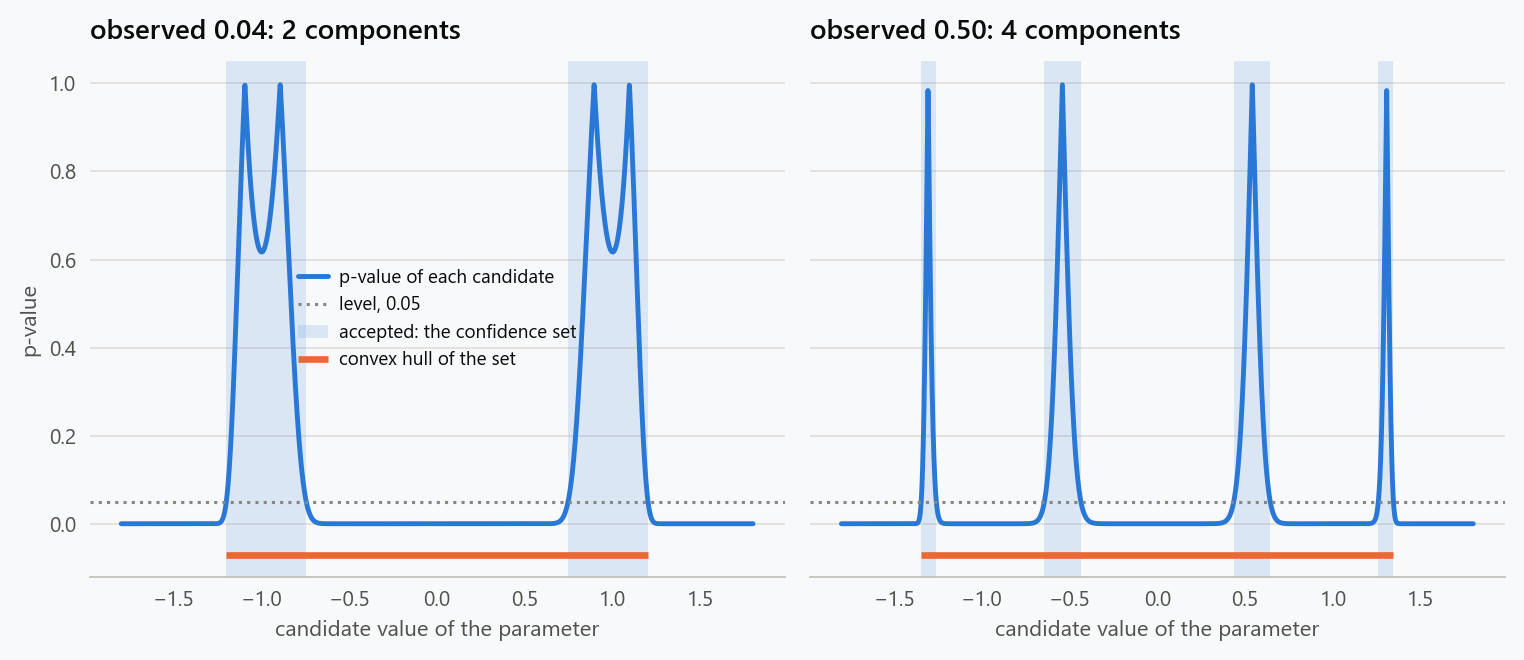
The figure shows the p-value curve for two of the rows. For $y = 0.04$ each component has two peaks, at the candidates whose mean equals the observation exactly, with a dip to $p = 0.62$ at $\theta = \pm 1$ where the mean is zero. Between the components the curve is flat at zero: at $\theta = 0$ the mean is 1, the observation is twelve standard deviations away, and the p-value is $4 \times 10^{-33}$. For $y = 0.50$ the lower bound in $\eqref{eq:accept}$ becomes active, values of $\theta$ near $\pm 1$ are rejected as well, and each component splits in two.
The empty row deserves a comment, because interval thinking has no place for it. When $y < -z\sigma$ no candidate has a mean close enough to the observation, every test rejects, and the set is empty. Under the true values $\theta = \pm 1$ this happens with probability exactly $\Phi(-1.96) = 0.025$. An empty set is not a malfunction. It says the observation is improbable under every parameter value, which is the 5% error the procedure is allowed, or evidence that the model is wrong. Software that repairs it, by returning the whole range or the least-rejected point, replaces that message with a fiction.
The Hull Is Valid, and It Says Less
The smallest interval containing the set for $y = 0.04$ is $[-1.20, 1.20]$. It is tempting to report it, and the first thing to be clear about is what goes wrong. The hull contains the set, so it covers the truth at least as often: it is a valid confidence set. What it loses is information. It is 2.6 times as long as the set it replaces, and it asserts compatibility with $\theta = 0$, the most thoroughly rejected value on the line. A simulation of 20,000 data sets at each of three true values makes the trade explicit.
| True $\theta$ | Coverage, set | Coverage, hull | Mean measure, set | Mean length, hull | Components: probability |
|---|---|---|---|---|---|
| $1.0$ | 95.1% | 97.5% | 0.77 | 2.30 | 0: 2.5%, 2: 95.1%, 4: 2.4% |
| $0.0$ | 95.2% | 100% | 0.66 | 2.88 | 2: 2.4%, 3: 95.2%, 4: 2.4% |
| $1.3$ | 95.2% | 97.6% | 0.60 | 2.68 | 4: 100% |
The set delivers its nominal 95% and the hull over-covers, in one case always, at three to four and a half times the size. If negative and positive values of $\theta$ correspond to different mechanisms and values near zero to no effect at all, the set says that either mechanism is supported and the null explanation is not. The hull says nothing of the kind.
None of this is peculiar to a toy. The oldest example is Fieller's (1954) confidence set for a ratio of two normal means $a/b$, obtained by inverting the test of $a - \rho b = 0$. It is the solution set of a quadratic inequality in $\rho$ whose leading coefficient is $\hat b^2 - z^2 s_b^2$, so its shape depends on whether the denominator is significantly different from zero. With $\hat a = 1$ and standard errors of $0.3$, a denominator of $\hat b = 2$ gives the interval $[0.20, 0.89]$; $\hat b = 0.5$ gives $(-\infty, -11.06] \cup [0.62, \infty)$, the complement of an interval; and with $\hat a = 0.2$, $\hat b = 0.3$ the set is the whole real line. Anderson and Rubin's (1949) sets for a structural coefficient behave the same way when instruments are weak (Staiger and Stock, 1997), and this is forced, not a defect of the method. Gleser and Hwang (1987) show that in such models no confidence set with positive coverage can have finite expected diameter, and Dufour (1997) that a valid set must be unbounded with positive probability. A procedure that always returns a bounded interval there cannot have the coverage it claims.
What a Grid Can and Cannot Establish
Few tests invert in closed form, so in practice the set is computed on a grid $\theta_1 < \dots < \theta_K$ and what the software holds is the finite set ${\theta_k : p(\theta_k) > \alpha}$. Runs of consecutive accepted points are a natural way to summarise it, and they are bookkeeping, not topology. Two accepted neighbours establish nothing about the values between them unless something is known about the smoothness of $p$, and two rejected neighbours establish nothing about a component lying entirely between them.
How easily is a component missed? One of width $w$ contains no grid point with probability $1 - w/h$ when the grid has step $h > w$ and an offset unrelated to the problem. In the four-component case above the outer pieces are $0.086$ wide and the inner ones $0.208$.
| Grid step | Misses an outer piece (0.086) | Misses an inner piece (0.208) | Misses a piece of the $y = 0.04$ set (0.456) |
|---|---|---|---|
| 0.05 | 0% | 0% | 0% |
| 0.10 | 14% | 0% | 0% |
| 0.20 | 57% | 0% | 0% |
| 0.50 | 83% | 58% | 9% |
A step that looks fine for one observation loses pieces for another, from the same model. The step has to be chosen against the narrowest component the procedure can produce, and when that is unknown the honest description of the output is "accepted grid points", not "the confidence set".
Refinement sharpens what the grid found and cannot find what it missed. Bisection between an accepted and a rejected neighbour localises that one transition; it says nothing about intervals whose ends agree. It also has a floor. Starting from $[0.5, 1]$ and bisecting towards the boundary of the $y = 0.04$ set, the computed midpoint equals one of the endpoints after 52 halvings, at a width of $1.1 \times 10^{-16}$ and a boundary of $0.745910039589340$. Adjacent double-precision numbers have no representable midpoint, so a tolerance below that spacing can never be met. An implementation should report that state as stalled, not as converged, because the loop ended for a reason unrelated to the tolerance the user asked for.
A third error source is independent of both. If $p(\theta)$ is itself a Monte Carlo estimate from $B$ draws, its standard error near $\alpha = 0.05$ is $\sqrt{0.05 \times 0.95 / B}$, which is $0.0069$ for $B = 999$. Candidates whose true p-value lies within about $0.014$ of the level are then accepted or rejected more or less at random, and no refinement of the grid helps: a bracket of width $10^{-6}$ around a noisy decision is a precise statement about the noise. Grid error, floating-point limits and Monte Carlo error need separate fields in a result, because they have separate remedies.
Nuisance Parameters: a Maximum Is Not a Supremum
With a parameter $(\psi, \lambda)$, target $\psi$ and nuisance $\lambda$, the joint set $\mathcal{C} = {(\psi, \lambda) : p(\psi, \lambda) > \alpha}$ is projected to the values of $\psi$ that some nuisance value makes acceptable. Equivalently, $\psi$ is accepted when the profile p-value
exceeds $\alpha$. The direction of the error matters here. Anything that returns less than the supremum makes the profile p-value too small, rejects target values that should be accepted, and produces a set that is too narrow. Computational shortcuts in this step are anti-conservative.
Take $Y \sim N(\psi + g(\lambda), \sigma^2)$ with $g(\lambda) = (\lambda^2 - 1)^2 - 0.3\lambda$, $\sigma = 0.06$ and $y = 0$. The function $g$ has two basins, a shallow one near $\lambda = -0.96$ where $g = 0.294$ and a deep one near $\lambda = 1.04$ where $g = -0.305$, and the supremum of the p-value is attained where $\psi + g(\lambda)$ comes closest to $y$. The projected set is therefore $\psi < 0.305 + 1.96\sigma = 0.423$.
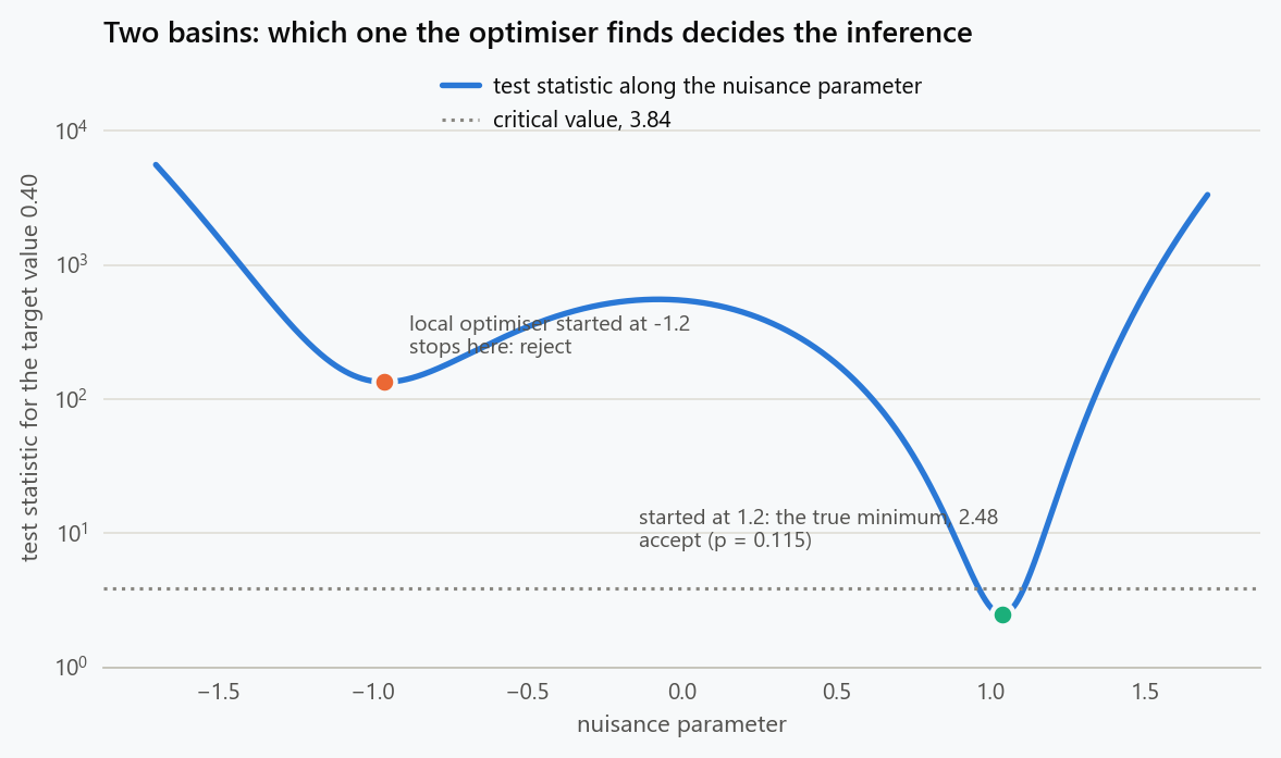
For the target value $\psi = 0.40$, a quasi-Newton optimiser started at $\lambda = -1.2$ converges, correctly, to the bottom of the left basin. The statistic there is $133.8$, the p-value is $6 \times 10^{-31}$, and the target is rejected. Started at $0$ or at $1.2$ it finds the right basin, a statistic of $2.48$ and a p-value of $0.115$: accepted. Nothing warned of the difference, because a local optimiser reports a local optimum and both runs converged. Used for every target value from the left start, it returns the set $\psi < -0.177$ and silently discards the interval $(-0.177, 0.423)$.
A finite grid over the nuisance parameter is limited in the same direction, but it is honest about it. Its maximum is an exact statement about the rows that were evaluated, and it can only understate the supremum. At $\psi = 0.42$ the supremum is $0.056$, so the value belongs to the set. A nuisance grid of step $0.5$ or $0.1$ returns $0.046$ and rejects it; a step of $0.05$ returns $0.054$ and accepts. The remedy is a finer grid or a global search with a guarantee, and the important thing is that the result object says which was used. "Maximum over 41 represented nuisance values" is a claim a reader can check. "Profile p-value" invites them to assume a supremum that was never computed. The same care applies to coverage: a guarantee proved for parameter vectors on the grid does not extend to values off it without an argument about what happens in between. In moment-inequality models, where this step is unavoidable, the choice between projecting a joint set and profiling a test is a research question in its own right (Bugni, Canay and Shi, 2017; Kaido, Molinari and Stoye, 2019).
That literature is also where the set view stops being a computational nicety. When a model is partially identified, the population object is itself a set, the identified set $\Theta_I = {\theta : E[m_j(W, \theta)] \le 0 \text{ for all } j}$, and it need be neither convex nor connected (Manski, 2003; Chernozhukov, Hong and Tamer, 2007). Confidence statements can target the set or the parameter inside it, which are different problems with different critical values (Imbens and Manski, 2004), and inference is by test inversion almost without exception (Andrews and Soares, 2010). Forcing the answer into an interval there discards the structure the model was built to reveal.
What Software Should Return
A result that respects the geometry keeps the evidence and the summary apart. For a one-dimensional inversion that means the candidates evaluated, their p-values or decisions, the accepted values, the runs of accepted neighbours, the level, the test and its Monte Carlo settings, the bounds of the search, and for each refined transition a bracket with a status that distinguishes converged from stalled. For a projection it adds the target values represented, the finite maximum for each, and a witness: one nuisance row attaining that maximum, which answers the question of what made a target value plausible. A convex hull is a reasonable thing to offer as well, provided it is named as a description of the range and is not the only thing returned.
Several properties are worth testing directly, because example-based tests rarely catch their violation. Permuting the rows of a parameter grid must not change the accepted values, the profile maxima or the components. The witness may change its row number under a permutation, so the invariant to assert is that it belongs to the right target group and attains the same maximum, not that its index is stable. An empty set and a one-point set must come back as such, without a fabricated pair of endpoints. And when the target is a transformation $\psi = h(\theta)$, the rule for deciding that two rows share a target value has to be explicit. Grouping by exact floating-point equality treats $0.1 + 0.2$ and $0.3$ as different targets, since the first is $0.30000000000000004$. Grouping within a tolerance is a different contract with different sets as output. Either can be right, and neither should happen by accident.
The plot to default to is the one in the first figure: the p-value of each candidate against the candidate, with a line at the level. The set is the region above the line, gaps and all, and on a coarse grid drawing the evaluated points instead of a filled band shows exactly how much was established.
The Geometry Is Part of the Result
Two analysts who report $[-1.2, 1.2]$ and $\pm(0.75, 1.20)$ for the same parameter agree on the range and disagree on the science. The second has ruled out a neighbourhood of zero at twelve standard deviations, and the first has hidden that. Deriving the set first and summarising it second costs little: a few more fields in a result, a plot with a horizontal line, and wording that distinguishes a maximum over a grid from a supremum over a continuum. What it buys is a statement of uncertainty that still means what the test said.
References
- Anderson, T. W., & Rubin, H. (1949). Estimation of the parameters of a single equation in a complete system of stochastic equations. The Annals of Mathematical Statistics, 20(1), 46-63.
- Andrews, D. W. K., & Soares, G. (2010). Inference for parameters defined by moment inequalities using generalized moment selection. Econometrica, 78(1), 119-157.
- Bugni, F. A., Canay, I. A., & Shi, X. (2017). Inference for subvectors and other functions of partially identified parameters in moment inequality models. Quantitative Economics, 8(1), 1-38.
- Casella, G., & Berger, R. L. (2002). Statistical Inference (2nd ed.). Duxbury.
- Chernozhukov, V., Hong, H., & Tamer, E. (2007). Estimation and confidence regions for parameter sets in econometric models. Econometrica, 75(5), 1243-1284.
- Dufour, J.-M. (1997). Some impossibility theorems in econometrics with applications to structural and dynamic models. Econometrica, 65(6), 1365-1387.
- Fieller, E. C. (1954). Some problems in interval estimation. Journal of the Royal Statistical Society: Series B, 16(2), 175-185.
- Gleser, L. J., & Hwang, J. T. (1987). The nonexistence of $100(1-\alpha)\%$ confidence sets of finite expected diameter in errors-in-variables and related models. The Annals of Statistics, 15(4), 1351-1362.
- Imbens, G. W., & Manski, C. F. (2004). Confidence intervals for partially identified parameters. Econometrica, 72(6), 1845-1857.
- Kaido, H., Molinari, F., & Stoye, J. (2019). Confidence intervals for projections of partially identified parameters. Econometrica, 87(4), 1397-1432.
- Manski, C. F. (2003). Partial Identification of Probability Distributions. Springer.
- Staiger, D., & Stock, J. H. (1997). Instrumental variables regression with weak instruments. Econometrica, 65(3), 557-586.
Embed interactive plots, widgets, and demos using <figure>, <iframe>, or <div class="interactive-embed"> containers. Ensure each embed includes descriptive captions for accessibility.
How to cite
Use the quick export buttons to save citations for reference managers or copy the formatted text directly.
Diogo Ribeiro (2026). Confidence Sets Are Not Just Intervals. Faculty of Media Arts and Design, Technical University of Porto. https://diogoribeiro7.github.io/statistics/confidence_sets_are_not_just_intervals/.

