Topics
Two reviewers worked through the same release independently. One logged 313 problems, the other 237, and 153 of them appear on both lists. The release meeting wants to know whether it is safe to ship, which is a question about the problems that are not on either list.
That number is estimable, and the overlap is what estimates it. If the second reviewer found 45 percent of everything, they should also have found about 45 percent of the first reviewer's list. Comparing the share of the first list they recovered against the size of the first list gives the total. The idea comes from counting fish, and it works equally well on defects, on duplicate records, on incidents that were never logged, and on any population sampled twice.
The Overlap Carries the Answer
The simulation puts 500 defects in a release and sends two reviewers through it, each finding a fixed share at random. Two estimators are compared: the textbook Lincoln-Petersen ratio, and Chapman's correction, which adds one to each count and is nearly unbiased in small samples.
1
2
3
4
5
6
7
8
9
10
11
12
13
14
15
16
17
18
19
20
21
22
23
24
25
26
27
28
29
30
31
32
33
34
35
36
37
38
39
40
41
42
43
44
45
46
47
import numpy as np

RNG = np.random.default_rng(11)
TRUE_N = 500          # defects actually present
REPS = 2000


def two_passes(n, p1, p2, spread=0.0, rng=RNG):
    """Two independent passes over n items. `spread` makes items differ in how
    easy they are to find, which correlates the two passes without either
    reviewer knowing the other's result."""
    if spread:
        ease = rng.lognormal(-spread ** 2 / 2, spread, n)
        q1 = np.clip(p1 * ease, 0, 1)
        q2 = np.clip(p2 * ease, 0, 1)
    else:
        q1 = np.full(n, p1)
        q2 = np.full(n, p2)
    a = rng.random(n) < q1
    b = rng.random(n) < q2
    return a, b


def lincoln(a, b):
    """Lincoln-Petersen: found by both is to found by one as found by the other
    is to the total."""
    n1, n2, m = a.sum(), b.sum(), (a & b).sum()
    return np.inf if m == 0 else n1 * n2 / m


def chapman(a, b):
    """Chapman's small-sample correction, which is nearly unbiased and always finite."""
    n1, n2, m = a.sum(), b.sum(), (a & b).sum()
    return (n1 + 1) * (n2 + 1) / (m + 1) - 1


def chapman_se(a, b):
    n1, n2, m = a.sum(), b.sum(), (a & b).sum()
    var = ((n1 + 1) * (n2 + 1) * (n1 - m) * (n2 - m)) / ((m + 1) ** 2 * (m + 2))
    return np.sqrt(var)


a, b = two_passes(TRUE_N, 0.60, 0.45)
print(f"reviewer A found {a.sum()}, reviewer B found {b.sum()}, both found {(a & b).sum()}")
print(f"union {(a | b).sum()}, so {TRUE_N - (a | b).sum()} defects were missed by both")
print(f"Lincoln-Petersen estimate {lincoln(a, b):.0f}, Chapman {chapman(a, b):.0f} "
      f"+- {chapman_se(a, b):.0f}, truth {TRUE_N}")
| Quantity | Value |
|---|---|
| Reviewer A found | 313 |
| Reviewer B found | 237 |
| Both found | 153 |
| On at least one list | 397 |
| On neither list | 103 |
| Lincoln-Petersen estimate | 485 |
| Chapman estimate | 484 ± 17 |
| Truth | 500 |
The estimate of 484 against a truth of 500 is one draw, and the interval covers the truth. What matters operationally is the difference between 397 and 484: the review found four fifths of what is there, and about 87 problems remain. Nobody had to know the detection rate in advance, because the overlap measures it.
The two estimators follow from one relation. With $n_1$ and $n_2$ found by each pass and $m$ in common,
Chapman's version exists because the first one divides by a random number that can be zero, and is biased upward when the overlap is small.
How Well It Behaves When Its Assumption Holds
1
2
3
4
5
6
7
8
9
10
11
12
13
14
15
16
for p1, p2 in ((0.60, 0.45), (0.40, 0.30), (0.25, 0.20)):
    lp, ch, cover, seen = [], [], [], []
    r = np.random.default_rng(3)
    for _ in range(REPS):
        a, b = two_passes(TRUE_N, p1, p2, rng=r)
        lp.append(lincoln(a, b))
        est, se = chapman(a, b), chapman_se(a, b)
        ch.append(est)
        cover.append(abs(est - TRUE_N) <= 1.96 * se)
        seen.append((a | b).sum())
    lp = np.array(lp)
    ch = np.array(ch)
    print(f"detection {p1:.0%} and {p2:.0%}: union sees {np.mean(seen):5.0f} of {TRUE_N}"
          f"   Lincoln-Petersen {np.median(lp):6.0f} (infinite in "
          f"{np.mean(~np.isfinite(lp)):.1%} of runs)"
          f"   Chapman {np.mean(ch):6.0f} +- {np.std(ch):4.0f}, covers {np.mean(cover):5.1%}")
| Detection rates | Seen by at least one pass | Lincoln-Petersen, median | Chapman, mean | Spread | Interval coverage |
|---|---|---|---|---|---|
| 60% and 45% | 390 | 499 | 499 | ±20 | 93.9% |
| 40% and 30% | 290 | 500 | 501 | ±43 | 94.3% |
| 25% and 20% | 200 | 500 | 501 | ±81 | 92.3% |
Both estimators are centred on the truth, and the interval keeps its coverage down to detection rates of one in five. The price of weak passes is width, not bias: at 25 and 20 percent the estimate carries a standard error of 81 on a population of 500, so it answers "between 340 and 660", which is still more than the 200 items on the lists.
The Assumption That Breaks It
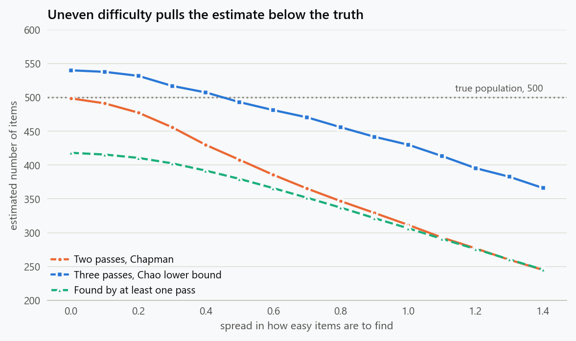
Everything above assumes every defect is equally likely to be found. Real defects are not like that. Some sit on the happy path and anyone would trip over them; others need a specific sequence on a specific device. When items differ in how easy they are to find, both reviewers tend to find the same easy ones, the overlap grows, and a large overlap reads as thorough coverage.
1
2
3
4
5
6
7
8
9
10
11
12
for spread in (0.0, 0.4, 0.8, 1.2):
    ch, seen, corr = [], [], []
    r = np.random.default_rng(5)
    for _ in range(REPS):
        a, b = two_passes(TRUE_N, 0.60, 0.45, spread=spread, rng=r)
        ch.append(chapman(a, b))
        seen.append((a | b).sum())
        # Correlation the heterogeneity induces between the two passes.
        corr.append(np.corrcoef(a.astype(float), b.astype(float))[0, 1])
    print(f"spread {spread:3.1f}: estimate {np.mean(ch):6.0f} (truth {TRUE_N}), "
          f"bias {np.mean(ch) / TRUE_N - 1:+6.1%}, union sees {np.mean(seen):5.0f}, "
          f"correlation between passes {np.mean(corr):+.3f}")
| Spread in how easy items are to find | Estimate | Bias | Seen by at least one pass | Correlation between passes |
|---|---|---|---|---|
| 0.0 | 501 | +0.1% | 390 | −0.001 |
| 0.4 | 439 | −12.2% | 367 | +0.149 |
| 0.8 | 359 | −28.1% | 313 | +0.328 |
| 1.2 | 288 | −42.4% | 254 | +0.441 |
The bias is always downward, and it is large. At the middle row the method reports 359 when the truth is 500, so a team that was told 46 problems remain would actually be facing 187. The failure is quiet: the two reviewers never communicated, so the passes look independent to anyone auditing the process, and the correlation is created by the defects rather than by the reviewers.
That correlation is measurable, and it is the warning sign. Cross-tabulate the two lists and compare the overlap against what independence predicts, which is $n_1 n_2 / N$. An overlap materially larger than that means the estimate is a lower bound rather than an estimate.
Using It to Decide Whether to Stop
The number a release meeting actually wants is not the total but the remainder: how many problems are still in there. That is the estimate minus what has been found, and its uncertainty is the estimate's uncertainty.
1
2
3
4
5
6
7
8
9
10
11
r = np.random.default_rng(7)
for p1, p2 in ((0.60, 0.45), (0.40, 0.30)):
    rows = []
    for _ in range(REPS):
        a, b = two_passes(TRUE_N, p1, p2, rng=r)
        est = chapman(a, b)
        rows.append((est - (a | b).sum(), TRUE_N - (a | b).sum()))
    rows = np.array(rows)
    print(f"detection {p1:.0%} and {p2:.0%}: estimated remaining {rows[:, 0].mean():5.1f} "
          f"+- {rows[:, 0].std():4.1f}, actually remaining {rows[:, 1].mean():5.1f} "
          f"+- {rows[:, 1].std():4.1f}")
| Detection rates | Estimated remaining | Actually remaining |
|---|---|---|
| 60% and 45% | 109.5 ± 16.5 | 110.2 ± 9.3 |
| 40% and 30% | 209.8 ± 38.3 | 209.9 ± 11.0 |
The estimate is centred on the truth in both rows, which is the useful property. Its spread is wider than the spread of the thing it estimates, which is the honest caveat: the method tells you the scale of what is left, not its exact size. For a release decision that is usually enough, because the decision changes between "about ten" and "about a hundred", not between 105 and 115.
What a Third Pass Buys
With two lists, independence has to be assumed. With three, there is enough information to model dependence between passes, by fitting a log-linear model to the seven observable combinations and extrapolating to the eighth. There is also Chao's estimator, which uses only the items seen exactly once and exactly twice, and which is a lower bound rather than a point estimate.
1
2
3
4
5
6
7
8
9
10
11
12
13
14
15
16
17
18
19
20
21
22
23
24
25
26
27
28
29
30
31
32
33
34
35
36
37
38
39
40
41
42
43
44
45
46
47
48
49
def three_passes(n, ps, spread, rng):
    ease = rng.lognormal(-spread ** 2 / 2, spread, n) if spread else np.ones(n)
    return [rng.random(n) < np.clip(p * ease, 0, 1) for p in ps]


def loglinear(a, b, c):
    """Fit a log-linear model with all pairwise interactions to the seven
    observable cells and read the missing one off the intercept."""
    obs, x, y = [], [], []
    for ia, va in ((1, a), (0, ~a)):
        for ib, vb in ((1, b), (0, ~b)):
            for ic, vc in ((1, c), (0, ~c)):
                if (ia, ib, ic) == (0, 0, 0):
                    continue
                n = int((va & vb & vc).sum())
                if n > 0:
                    x.append([1, ia, ib, ic, ia * ib, ia * ic, ib * ic])
                    y.append(np.log(n))
                obs.append(n)
    beta, *_ = np.linalg.lstsq(np.array(x, float), np.array(y, float), rcond=None)
    return sum(obs) + np.exp(beta[0])


def chao(a, b, c):
    """Chao's lower bound: items seen once and twice carry the information about
    items seen never, and it does not assume the passes are independent. With t
    passes the correction carries a factor (t - 1) / t."""
    t = 3
    times = a.astype(int) + b.astype(int) + c.astype(int)
    d = int((times > 0).sum())
    f1 = int((times == 1).sum())
    f2 = int((times == 2).sum())
    return d + (t - 1) / t * f1 ** 2 / (2 * f2) if f2 else np.inf


for spread in (0.0, 0.4, 0.8, 1.2):
    pair, tri, ch3, seen = [], [], [], []
    r = np.random.default_rng(13)
    for _ in range(1000):
        a, b, c = three_passes(TRUE_N, (0.5, 0.45, 0.4), spread, r)
        pair.append(chapman(a, b))
        tri.append(loglinear(a, b, c))
        ch3.append(chao(a, b, c))
        seen.append(int((a | b | c).sum()))
    print(f"spread {spread:3.1f}: union {np.mean(seen):5.0f}   "
          f"two passes {np.median(pair):6.0f}   "
          f"three passes, interactions {np.median(tri):6.0f} "
          f"(quartiles {np.percentile(tri, 25):.0f} to {np.percentile(tri, 75):.0f})   "
          f"Chao lower bound {np.median(ch3):6.0f}   truth {TRUE_N}")
| Spread | Seen by any pass | Two passes | Three passes with interactions | Chao lower bound |
|---|---|---|---|---|
| 0.0 | 418 | 497 | 498, quartiles 482 to 520 | 501 |
| 0.4 | 393 | 434 | 535, quartiles 503 to 576 | 470 |
| 0.8 | 338 | 348 | 714, quartiles 618 to 839 | 419 |
| 1.2 | 276 | 277 | 952, quartiles 755 to 1205 | 359 |
The truth is 500 in every row. When the passes really are independent, all three methods agree and the log-linear model costs nothing. As soon as items differ in difficulty, the two-pass estimate collapses downward and the log-linear model overshoots, badly and with enormous spread, because it is fitting a pairwise interaction to a dependence that is not pairwise: the passes are correlated through the items, not through each other. Chao's bound stays closest, and errs in the direction it is meant to, which is low.
That is the practical hierarchy. Three lists are worth having, but the extra list buys a diagnostic more reliably than it buys a better point estimate. When the overlap is larger than independence predicts, quote Chao's number as a floor and say so.
Where This Gets Used
The same arithmetic answers several questions that otherwise get guessed. How many duplicate records are in a table, from two different matching rules run independently. How many incidents went unlogged, from an on-call log and a customer complaint log. How many errors are in a dataset, from two annotators checking different samples. How many users hit a bug, from support tickets and error telemetry.
Each of those has the same weakness. Two matching rules both find the obvious duplicates; both logs record the severe incidents; both annotators spot the blatant errors. The bias is always in the same direction, and it is always reassuring, which is the worst combination.
What to Do
- Run the two passes genuinely independently. If the second reviewer sees the first one's list, the overlap is manufactured and the estimate is meaningless.
- Use Chapman's form rather than the plain ratio. It cannot divide by zero and it is nearly unbiased at the sample sizes reviews actually produce.
- Compare the observed overlap against the product of the two list sizes divided by the estimate. A materially larger overlap means the items differ in difficulty and the estimate is a floor.
- Report the remainder with its interval, not just the point estimate. The decision usually rests on the order of magnitude, which the method gives reliably.
- Add a third pass when the stakes justify it, and use it first to test dependence rather than to refine the number.
- When dependence is present, quote Chao's lower bound and describe it as a lower bound. A floor that is honest beats a point estimate that is quietly 30 percent low.
The figure generator in the blog-reproducibility repository reproduces this article's figure; run it with --dry-run to print the numbers behind the figure without writing an image.
References
- Chapman, D. G. (1951). Some properties of the hypergeometric distribution with applications to zoological sample censuses. University of California Publications in Statistics, 1(7), 131-160.
- Chao, A. (1987). Estimating the population size for capture-recapture data with unequal catchability. Biometrics, 43(4), 783-791.
- Seber, G. A. F. (1982). The Estimation of Animal Abundance and Related Parameters. Macmillan.
- Hook, E. B., & Regal, R. R. (1995). Capture-recapture methods in epidemiology: methods and limitations. Epidemiologic Reviews, 17(2), 243-264.
- International Working Group for Disease Monitoring and Forecasting (1995). Capture-recapture and multiple-record systems estimation I: history and theoretical development. American Journal of Epidemiology, 142(10), 1047-1058.
- Eick, S. G., Loader, C. R., Long, M. D., Votta, L. G., & Vander Wiel, S. (1992). Estimating software fault content before coding. Proceedings of the 14th International Conference on Software Engineering, 59-65.
Embed interactive plots, widgets, and demos using <figure>, <iframe>, or <div class="interactive-embed"> containers. Ensure each embed includes descriptive captions for accessibility.
How to cite
Use the quick export buttons to save citations for reference managers or copy the formatted text directly.
Diogo Ribeiro (2025). Capture-Recapture: Counting the Defects Both Reviews Missed. Faculty of Media Arts and Design, Technical University of Porto. https://diogoribeiro7.github.io/statistics/capture_recapture_estimating_what_was_missed/.

