Topics
A supplier delivers ten thousand parts. Quality control inspects fifty, finds nothing wrong, and the delivery is accepted. The same routine appears in data work: a new feed arrives, an analyst checks a hundred rows, everything looks right, the feed goes live.
Neither check establishes what people take from it. A batch running at two percent defective passes an inspection of fifty with nothing found 36 percent of the time. The inspection did not show the batch was clean. It showed the batch was not disastrous, which is a much weaker claim, and the arithmetic that says how much weaker has been settled since the 1920s.
What a Clean Sample Rules Out
A sample of $n$ with no defects is consistent with any rate low enough that $n$ clean draws are unremarkable. The highest rate that would still produce a clean sample five percent of the time is the useful bound, and it falls only as fast as $1/n$.
1
2
3
4
5
6
7
8
9
10
11
12
13
14
15
16
import numpy as np
from scipy import stats

RNG = np.random.default_rng(41)


def accept_prob(n, c, p):
    """Chance a lot with defect rate p passes a plan that inspects n and
    allows at most c defects."""
    return stats.binom.cdf(c, n, p)


for n in (20, 50, 100, 300, 1000):
    p95 = 1 - 0.05 ** (1 / n)          # highest rate that still passes 5% of the time
    print(f"inspect {n:5d}, find none: rates above {p95:6.2%} are rejected 95% of the time, "
          f"and a lot at {p95 / 2:6.2%} passes {accept_prob(n, 0, p95 / 2):5.1%} of the time")
| Inspected, none defective | Rates rejected 95% of the time | A lot at half that rate still passes |
|---|---|---|
| 20 | above 13.91% | 23.6% of the time |
| 50 | above 5.82% | 22.9% of the time |
| 100 | above 2.95% | 22.6% of the time |
| 300 | above 0.99% | 22.4% of the time |
| 1,000 | above 0.30% | 22.4% of the time |
Fifty clean items rule out rates above about six percent and say nothing about anything below three. That is the honest reading of the routine inspection, and it is the same rule of three that governs any zero-count observation: the upper bound is roughly three divided by the sample size.
The Operating Characteristic
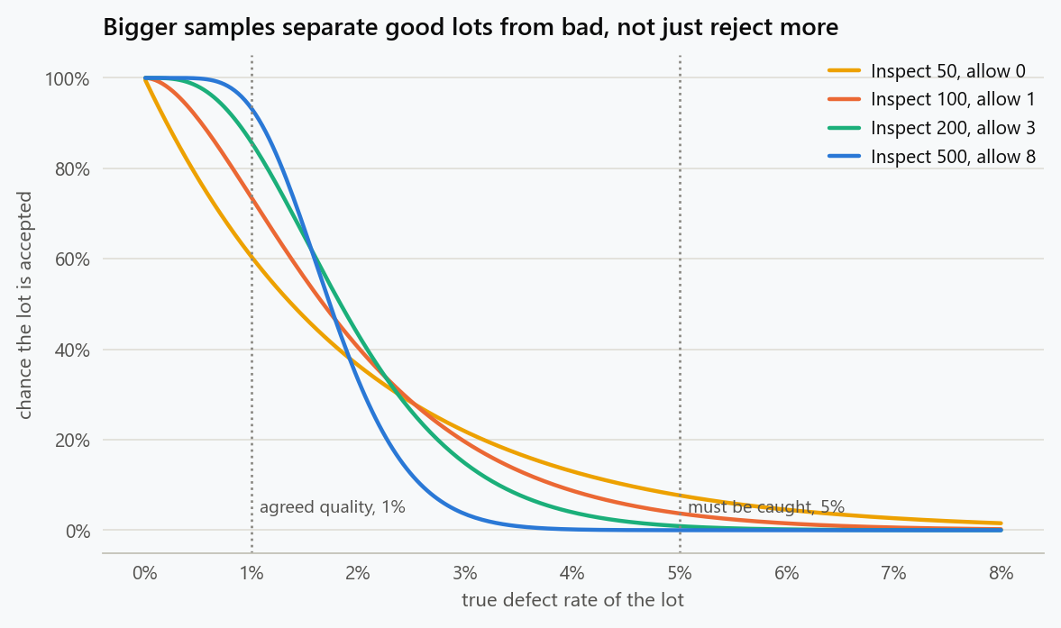
A plan is a pair: inspect $n$, accept if at most $c$ are defective. Its operating characteristic is the chance of acceptance at each true rate, and it is what makes two plans comparable.
1
2
3
4
5
6
7
plans = [(50, 0), (100, 1), (200, 3), (500, 8)]
rates = (0.001, 0.005, 0.01, 0.02, 0.05)
header = "  plan      " + "".join(f"{r:>10.1%}" for r in rates)
print(header)
for n, c in plans:
    row = "".join(f"{accept_prob(n, c, r):>10.1%}" for r in rates)
    print(f"  n={n:<4d} c={c:<2d}{row}")
| Plan | 0.1% | 0.5% | 1.0% | 2.0% | 5.0% |
|---|---|---|---|---|---|
| Inspect 50, allow 0 | 95.1% | 77.8% | 60.5% | 36.4% | 7.7% |
| Inspect 100, allow 1 | 99.5% | 91.0% | 73.6% | 40.3% | 3.7% |
| Inspect 200, allow 3 | 100.0% | 98.1% | 85.8% | 43.1% | 0.9% |
| Inspect 500, allow 8 | 100.0% | 99.9% | 93.3% | 33.1% | 0.0% |
Read the columns rather than the rows. Every plan here accepts a one-in-a-thousand lot and rejects a five-percent lot, and they differ in the middle, which is where real suppliers live. The first plan rejects four good lots in ten at a one percent rate; the last accepts nine in ten. Larger samples buy discrimination, not severity: the bottom row is both kinder to good lots and harsher on bad ones.
Choosing a Plan From Two Risks
The design question is not "how many should we check" but "which two rates matter". An acceptable quality level is the rate a good supplier should almost always pass; a tolerance level is the rate that must almost always be caught. Fix those two and the plan follows.
1
2
3
4
5
6
7
8
9
10
11
12
AQL, LTPD = 0.01, 0.05      # acceptable rate, and the rate that must be caught
print(f"accept 95% of lots at {AQL:.0%}, reject 90% of lots at {LTPD:.0%}")
best = None
for c in range(0, 12):
    n = c + 1
    while n < 5000:
        if accept_prob(n, c, AQL) >= 0.95 and accept_prob(n, c, LTPD) <= 0.10:
            print(f"  c = {c:2d}: n = {n:4d}   passes at AQL {accept_prob(n, c, AQL):5.1%}, "
                  f"passes at LTPD {accept_prob(n, c, LTPD):5.1%}")
            best = best or (n, c)
            break
        n += 1
| Accept number | Smallest sample that meets both risks | Passes at 1% | Passes at 5% |
|---|---|---|---|
| 3 | 132 | 95.6% | 9.9% |
| 4 | 158 | 97.8% | 10.0% |
| 5 | 184 | 98.9% | 9.8% |
| 6 | 209 | 99.5% | 9.8% |
| 8 | 258 | 99.9% | 9.9% |
| 11 | 330 | 100.0% | 9.8% |
Accept numbers of zero, one and two appear nowhere in the table, because no sample size satisfies both constraints with them. That is the central and least intuitive result here: a stricter rule does not make a better plan. The smallest plan meeting both risks inspects 132 and tolerates three defects.
The Price of Zero Tolerance
Zero-defect rules are popular because they sound rigorous. What they actually do is shift the entire burden onto the supplier's good batches.
1
2
3
4
for c, n in ((0, 45), (1, 77), (2, 105), (3, 132)):
    print(f"c = {c}, n = {n:3d}: passes at 1% {accept_prob(n, c, 0.01):5.1%}, "
          f"passes at 5% {accept_prob(n, c, 0.05):5.1%}, "
          f"producer's risk at 1% {1 - accept_prob(n, c, 0.01):5.1%}")
| Plan | Passes at 1% | Passes at 5% | Good lots wrongly rejected |
|---|---|---|---|
| Inspect 45, allow 0 | 63.6% | 9.9% | 36.4% |
| Inspect 77, allow 1 | 82.0% | 9.7% | 18.0% |
| Inspect 105, allow 2 | 91.1% | 9.9% | 8.9% |
| Inspect 132, allow 3 | 95.6% | 9.9% | 4.4% |
All four plans are equally severe on a five-percent lot, catching ninety percent of them. They differ entirely in what they do to a supplier running at one percent, which the contract calls acceptable: the zero-tolerance plan rejects more than a third of those batches, the tolerant plan one in twenty-three. The cost of those false rejections lands as returned shipments, expedited replacements and an adversarial relationship with a supplier who is meeting the agreement.
Two Stages Instead of One
Most lots are clearly fine or clearly bad, and only the ambiguous ones need a full inspection. A two-stage plan exploits that: inspect a first sample, accept immediately if it is clean enough, reject immediately if it is bad enough, and inspect more only in between.
1
2
3
4
5
6
7
8
9
10
11
12
13
14
15
16
17
18
def double_plan(p, n1, c1, r1, n2, c2, rng, reps=20000):
    """Inspect n1. Accept at c1 or fewer, reject at r1 or more, otherwise
    inspect n2 more and judge on the total."""
    first = rng.binomial(n1, p, reps)
    decided = (first <= c1) | (first >= r1)
    second = rng.binomial(n2, p, reps)
    total = first + second
    accept = np.where(decided, first <= c1, total <= c2)
    inspected = np.where(decided, n1, n1 + n2)
    return accept.mean(), inspected.mean()


single_n, single_c = 132, 3
for p in (0.005, 0.01, 0.02, 0.05):
    acc_d, avg_n = double_plan(p, 80, 1, 4, 80, 4, np.random.default_rng(3))
    print(f"true rate {p:5.1%}: single plan n={single_n} accepts "
          f"{accept_prob(single_n, single_c, p):5.1%} inspecting {single_n} every time; "
          f"double plan accepts {acc_d:5.1%} inspecting {avg_n:5.0f} on average")
| True defect rate | Single plan accepts | Items inspected | Two-stage plan accepts | Items inspected on average |
|---|---|---|---|---|
| 0.5% | 99.5% | 132 | 99.8% | 85 |
| 1.0% | 95.6% | 132 | 97.8% | 95 |
| 2.0% | 72.8% | 132 | 79.8% | 112 |
| 5.0% | 9.9% | 132 | 13.8% | 107 |
At the rate a good supplier runs, the two-stage plan inspects 95 items instead of 132, a 28 percent saving, while accepting slightly more often. The saving is largest exactly where most lots sit. The cost is a little less discrimination at the bad end, 13.8 percent acceptance instead of 9.9, which can be tuned back by tightening the second-stage accept number.
When the Lot Is Small
The binomial calculation assumes each inspected item is drawn from an unchanged population, which is fine for a lot of ten thousand and wrong for a lot of two hundred.
1
2
3
4
5
6
for lot in (200, 500, 2000, 100000):
    n, c, defects = 50, 0, int(round(0.02 * lot))
    hyper = stats.hypergeom.cdf(c, lot, defects, n)
    binom = accept_prob(n, c, 0.02)
    print(f"lot of {lot:6d} with 2% defective: exact {hyper:6.2%}, "
          f"binomial approximation {binom:6.2%}, difference {hyper - binom:+.2%}")
| Lot size | Exact acceptance probability | Binomial approximation | Difference |
|---|---|---|---|
| 200 | 31.32% | 36.42% | −5.10% |
| 500 | 34.52% | 36.42% | −1.90% |
| 2,000 | 35.96% | 36.42% | −0.46% |
| 100,000 | 36.41% | 36.42% | −0.01% |
The approximation errs in the safe direction, overstating the chance a bad lot passes, and the error is worth carrying only when the sample is a substantial fraction of the lot. A practical rule: use the exact calculation when the sample exceeds about a tenth of the lot.
The Same Arithmetic for a Data Audit
None of this is specific to physical parts. Sampling rows from a table to check a transformation is the same problem with different vocabulary, and the sample sizes people use are just as habitual.
1
2
3
4
5
6
7
8
for rows, sample in ((2_000_000, 200), (2_000_000, 1000), (2_000_000, 5000)):
    for true_rate in (0.001, 0.005):
        r = np.random.default_rng(5)
        found = r.binomial(sample, true_rate, 20000)
        print(f"{rows:,} rows, sample {sample:5d}, true error rate {true_rate:.1%}: "
              f"finds nothing {np.mean(found == 0):5.1%} of the time, "
              f"expected errors in the sample {sample * true_rate:5.1f}, "
              f"implied errors in the table {rows * true_rate:8,.0f}")
| Sample size | True error rate | Audit finds nothing | Expected errors in the sample | Errors actually in the table |
|---|---|---|---|---|
| 200 | 0.1% | 81.7% | 0.2 | 2,000 |
| 200 | 0.5% | 37.1% | 1.0 | 10,000 |
| 1,000 | 0.1% | 37.1% | 1.0 | 2,000 |
| 1,000 | 0.5% | 0.6% | 5.0 | 10,000 |
| 5,000 | 0.1% | 0.6% | 5.0 | 2,000 |
| 5,000 | 0.5% | 0.0% | 25.0 | 10,000 |
Two hundred rows checked by hand is the most common data audit there is, and against a table carrying two thousand bad rows it comes back clean four times in five. The audit is not weak because the checker is careless; it is weak because 200 is the wrong number. Moving to a thousand rows changes the answer from "we found nothing" to "we expect to see about one, and we did".
The last column is the one to put in the report. A one-in-a-thousand error rate sounds tolerable and means two thousand broken rows, which may or may not be acceptable depending on what reads them.
What to Do
- State the two rates before choosing a sample size: the rate a good supplier or pipeline should pass, and the rate that must be caught. The plan follows from them.
- Stop using zero-defect acceptance as a default. It is the harshest plan on batches that meet the agreement and no harsher on the ones that do not.
- Publish the operating characteristic alongside the plan, so both sides can see what each rate implies rather than arguing about a single number.
- Use two-stage sampling when inspection is expensive. It typically cuts the average inspected by a quarter at the rates suppliers actually run.
- Switch to the exact finite-lot calculation when the sample exceeds about a tenth of the lot.
- Size data audits the same way, and report the implied number of affected rows rather than the rate. Two hundred rows finds nothing in a table with thousands of errors.
The figure generator in the blog-reproducibility repository reproduces this article's figure; run it with --dry-run to print the numbers behind the figure without writing an image.
References
- Dodge, H. F., & Romig, H. G. (1959). Sampling Inspection Tables: Single and Double Sampling (2nd ed.). Wiley.
- Schilling, E. G., & Neubauer, D. V. (2017). Acceptance Sampling in Quality Control (3rd ed.). CRC Press.
- Montgomery, D. C. (2019). Introduction to Statistical Quality Control (8th ed.). Wiley.
- Wald, A. (1947). Sequential Analysis. Wiley.
- Hanley, J. A., & Lippman-Hand, A. (1983). If nothing goes wrong, is everything all right? Interpreting zero numerators. JAMA, 249(13), 1743-1745.
- American Society for Quality (2018). ANSI/ASQ Z1.4: Sampling Procedures and Tables for Inspection by Attributes. ASQ.
Embed interactive plots, widgets, and demos using <figure>, <iframe>, or <div class="interactive-embed"> containers. Ensure each embed includes descriptive captions for accessibility.
How to cite
Use the quick export buttons to save citations for reference managers or copy the formatted text directly.
Diogo Ribeiro (2026). Acceptance Sampling: What a Clean Sample of Fifty Actually Proves. Faculty of Media Arts and Design, Technical University of Porto. https://diogoribeiro7.github.io/statistics/acceptance_sampling_what_a_clean_sample_proves/.

