Topics
The Northern and Southern Hemispheres experience opposite seasons while travelling around the Sun together. That observation is a useful test of the claim that summer happens simply because Earth is closer to the Sun.
Earth's distance does vary. But a change in the whole planet's orbital distance cannot, on its own, explain why one hemisphere moves into summer while the other moves into winter.
The central mechanism is Earth's tilted rotation axis. It changes how sunlight reaches different latitudes through the year. NASA's explanation of orbital cycles distinguishes this tilt from the effects of changing distance. NASA on tilt and orbit.
To see what tilt actually does, we can temporarily remove changing distance from the calculation.
The axis does not turn towards the Sun every morning
Earth rotates around an axis that is tilted relative to the direction perpendicular to its orbital plane. Over a single year, that axis points approximately in the same direction relative to distant stars. As Earth moves to the opposite side of its orbit, the hemisphere tilted towards the Sun becomes the hemisphere tilted away from it.
This geometry does not require the planet to rock back and forth each year. The annual change comes from moving a consistently tilted axis around the orbit. Daily rotation then carries each location through the illuminated and dark parts of the sphere.
It helps to distinguish two angles. Latitude locates a place north or south of the equator. Solar declination describes the latitude where the noon Sun is directly overhead. In the ideal geometry used here, declination varies from about 23.44° south at the December solstice to 23.44° north at the June solstice, crossing the equator at the equinoxes.
A place can keep exactly the same latitude while the Sun's declination changes. That combination determines the daily path of the Sun through its sky. Saying only that Earth is tilted skips this link between orbital geometry and what an observer actually experiences.
Give the model a circular orbit
Imagine a spherical Earth at a constant distance from the Sun. Give it an axial tilt of 23.44 degrees, a representative value close to Earth's present tilt.
Choose a location at 45 degrees north. Ignore mountains, clouds, atmospheric refraction, and the apparent width of the Sun. Treat sunrise and sunset as the moments when the centre of a point-like Sun crosses an unobstructed horizon.
Those assumptions simplify the arithmetic. They also tell us why the calculated daylight hours will differ slightly from a real sunrise table.
Now compare the December solstice, an equinox, and the June solstice:
| Idealised date | Sun's altitude at local noon | Daylight at 45° north |
|---|---|---|
| December solstice | 21.56° | 8.57 hours |
| Equinox | 45.00° | 12.00 hours |
| June solstice | 68.44° | 15.43 hours |
The distance to the Sun has not changed in this model. Both the height of the noon Sun and the length of the day have.
The same light spreads over different areas
Picture a beam of sunlight reaching a horizontal surface. When the Sun is overhead, the beam's cross-section covers the smallest area. At a shallow angle, the same beam spreads across a larger patch of ground.
For a horizontal surface, the incoming power per unit area is proportional to the sine of the Sun's altitude, before accounting for the atmosphere. The relevant question is the energy arriving on each square metre, not whether the sunlight has travelled a slightly longer distance across that square metre.
At the two solstices in our example:
- A noon altitude of 21.56° gives a projection factor of about 0.367.
- A noon altitude of 68.44° gives a projection factor of about 0.930.
At the higher angle, each horizontal square metre receives about 2.5 times as much instantaneous noon solar power in this idealisation. The incoming beam perpendicular to its own direction has the same intensity in both cases.
Noon is only one moment. We also need to add the sunlight arriving during the rest of the day.
A longer day changes the total
The winter day has about 8.6 hours of daylight; the summer day has about 15.4. The Sun also follows different paths above the horizon, so multiplying the noon value by daylight hours would not give the correct daily total.
Instead, we can integrate the changing projection through the day. To avoid introducing a particular value for solar intensity, express the result as equivalent hours of overhead sunlight. One such hour supplies the energy that a horizontal surface would receive in one hour with the Sun directly overhead, at the model's fixed distance.
| Idealised date | Daily incoming energy at 45° north |
|---|---|
| December solstice | 2.05 equivalent overhead hours |
| Equinox | 5.40 equivalent overhead hours |
| June solstice | 8.81 equivalent overhead hours |
The summer value is about 4.3 times the winter value. This is a comparison of ideal incoming energy, not a prediction that the air temperature becomes 4.3 times higher.
Repeat the calculation at 45 degrees south and the solstice values exchange places.
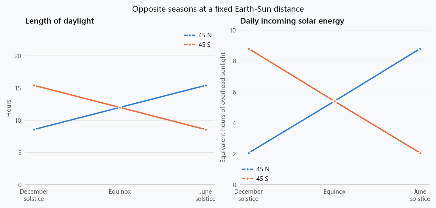
Original geometric calculation. Distance is fixed; atmospheric effects, terrain, and heat storage are omitted. The right panel integrates sunlight over the day rather than using only the noon angle.
This is the mechanism a distance-only account misses: the same orbital position can favour one hemisphere's sunlight geometry while disadvantaging the other's. NASA's satellite-based seasonal illustration shows the corresponding changes in how sunlight is distributed across Earth. Equinoxes and solstices from space.
Move the observer and the seasonal pattern changes
The 45° calculation describes one pair of latitudes. It is useful to check what the same mechanism predicts elsewhere, rather than assuming every place experiences the same seasonal contrast.
| Latitude | December daylight | June daylight | December energy, overhead hours | June energy, overhead hours |
|---|---|---|---|---|
| Equator | 12.00 h | 12.00 h | 7.01 | 7.01 |
| 45° north | 8.57 h | 15.43 h | 2.05 | 8.81 |
| 70° north | 0.00 h | 24.00 h | 0.00 | 8.97 |
These values use the same atmosphere-free sphere and fixed solar distance. At 70° north the ideal December Sun stays below the horizon, while the June Sun stays above it. The code handles those limiting cases by allowing zero or 24 hours of daylight instead of trying to calculate a sunrise that does not occur.
The polar summer result can seem surprising: why is its daily energy slightly higher than at 45° north when the noon Sun is lower? The lower instantaneous intensity is compensated by receiving sunlight around the full rotation. A lower peak and a longer duration can produce a larger accumulated total.
That result does not predict that the Arctic must be hotter than a temperate city in June. The surface does not receive the atmosphere-free energy in the table unchanged, and temperature depends on reflection, atmospheric processes, existing snow and ice, and stored heat. A geometric calculation of incoming energy cannot settle all of those processes.
The equator provides a different check. Both solstices have equal daylight and equal energy in this symmetric model. At an equinox, however, the noon Sun is directly overhead, and the daily total rises to about 7.64 equivalent overhead hours. The geometric annual cycle therefore has two maxima there. A simple Northern Hemisphere summer-versus-winter story does not describe every latitude equally well.
This is a useful property of a physical explanation: changing a clearly specified input, such as latitude, produces a testable change in the prediction. A diagram that merely labels one side of an ellipse “summer” does not supply that predictive structure.
Distance still has an effect
Removing distance changes from the model does not imply that distance is physically irrelevant. Solar intensity decreases with the square of distance from the Sun.
Earth is closest to the Sun in early January and farthest away in early July. The closer position therefore occurs during Northern Hemisphere winter, which is another difficulty for the simple “closer means northern summer” explanation. NASA describes the present orbital distance variation as roughly 3.4%. NASA orbital explanation.
An illustrative distance ratio of 1.034 would correspond to an intensity ratio of about $1.034^2=1.069$, or roughly a 7% difference. That affects the incoming energy budget. It does not replace the tilt mechanism demonstrated by the opposite-hemisphere calculation.
The two effects should therefore be separated rather than treating one as nonexistent. Tilt explains the alternating seasonal geometry. Distance modifies the amount of solar energy available to that geometry.
Why the hottest day does not have to be the longest
The calculation concerns incoming sunlight. Temperature reflects a continuing energy balance: energy arrives, energy leaves, and energy is stored and transported.
A simple analogy is filling a bath with the drain open. The moment when the tap runs fastest need not be the moment when the bath contains the most water. The amount in the bath depends on the accumulated difference between inflow and outflow.
Likewise, a solar-energy maximum does not by itself identify the warmest day. Clouds, atmospheric conditions, oceans, land, and geography matter for the temperature response. Our bare-sphere calculation deliberately cannot predict a particular location's seasonal lag or weather.
Its narrower achievement is enough to test the misconception. Opposite seasonal energy patterns emerge even with a fixed Earth-Sun distance, once the axis is tilted.
Put numbers on the delay caused by heat storage
We can take the bath analogy one step further without pretending to simulate a real climate. Consider a single hypothetical reservoir whose temperature departure from its annual mean is $\theta(t)$. It absorbs a smooth annual forcing and loses additional energy in proportion to that temperature departure:
Here $C$ is heat capacity per unit area, $\lambda$ describes how strongly the restoring energy loss changes with temperature, and $F$ is the amplitude of the seasonal energy input per unit area. The angular frequency is $\omega=2\pi/365$ when time is measured in days and the other units are made consistent. We have centred the forcing so its maximum occurs at $t=0$.
If heat storage were negligible, the temperature departure would follow the forcing immediately, with amplitude $F/\lambda$. With storage, the reservoir takes time to adjust. Its response time is $\tau=C/\lambda$.
After the initial transient has decayed, the periodic solution is
The formula separates two consequences. The factor in front of the cosine reduces the temperature amplitude. The phase angle shifts the temperature maximum later than the forcing maximum.
| Assumed response time $\tau$ | Amplitude relative to immediate equilibrium | Temperature maximum after forcing maximum |
|---|---|---|
| 10 days | 98.6% | 9.9 days |
| 30 days | 88.9% | 27.7 days |
| 90 days | 54.2% | 58.0 days |
For example, if the hypothetical immediate-equilibrium temperature amplitude were 10 degrees, the 90-day reservoir would vary with amplitude about 5.42 degrees and peak about 58 days later. Those are chosen model parameters, not measured values for an ocean or a city.
The delay has a physical interpretation. After incoming energy begins declining from its maximum, the reservoir can still be gaining energy overall. Its temperature continues to rise until the incoming and outgoing terms balance at that moment. The date of maximum input and the date of maximum stored energy answer different questions.
The calculation also explains why simply saying “the longest day should be the hottest” is incomplete. That statement silently assumes an immediate response and ignores the reservoir's existing state. Even this very small model breaks the assumed coincidence while keeping the energy accounting explicit.
Real seasonal forcing is not a perfect sinusoid, and the restoring term need not be linear. A real location exchanges energy with its surroundings and can contain several reservoirs with different response times. Those omissions prevent us from assigning the table's lags to a particular city. They do not prevent the model from showing how a lag can arise.
Turn a demonstration into a testable explanation
A globe and a fixed lamp can demonstrate the geometry if the rotation axis keeps its orientation while the globe travels around the lamp. Mark a latitude, rotate the globe at several orbital positions, and compare how much of the marked circle lies in light. The changing illuminated fraction represents changing daylight duration.
To demonstrate projection separately, hold a flat card in a fixed beam and tilt it. The same bundle of light covers a larger area when it strikes obliquely. Keep the beam and distance unchanged during that comparison; otherwise changing several things at once makes it harder to identify the cause.
Neither demonstration measures the temperature response. A lamp's nearby rays also diverge much more than sunlight across Earth, so the setup is an illustration with its own geometric limitations. The value comes from predicting what should change when the axis, latitude, or surface angle changes, then checking whether the demonstration behaves accordingly.
When evaluating a social-media animation, make the same distinctions. Does it show the axis keeping its orientation? Are the hemispheres treated consistently? Is a claim about sunlight being turned into a temperature claim without explaining storage and energy loss? These questions expose a missing mechanism more effectively than memorising the word “tilt.”
Try the explanation against a counterfactual
In the same model, remove the tilt as well as the distance variation. At 45 degrees north, every day then has the equinox geometry: a noon altitude of 45 degrees and 12 hours of daylight.
The annual alternation disappears from this model. That comparison identifies what the tilted axis contributed, while leaving the other assumptions unchanged.
When discussing the seasons, this is more useful than pointing only to an exaggerated ellipse in a diagram. Ask which feature of the explanation predicts opposite seasons in the hemispheres, and which quantities change when that feature is removed.
Follow the geometry
For latitude $\phi$ and solar declination $\delta$, the ideal sunset hour angle is
At the latitudes used in the table, daylight lasts $24H_0/\pi$ hours. The average incoming solar power over a complete day, as a fraction of the perpendicular beam intensity $S_0$, is
Multiplying this fraction by 24 gives the equivalent overhead hours. Angles inside the trigonometric functions are in radians. Polar day and night require the corresponding limiting cases, handled in the code.
The heat-storage table can be reproduced independently:
1
2
3
4
5
6
7
from math import atan, pi, sqrt

omega = 2 * pi / 365
for tau in (10, 30, 90):
    amplitude_fraction = 1 / sqrt(1 + (omega * tau)**2)
    lag_days = atan(omega * tau) / omega
    print(tau, f"amplitude={amplitude_fraction:.1%}; lag={lag_days:.1f} days")
The figure generator reproduces the geometry, latitude, and heat-storage tables. Its geometry is checked against direct numerical integration of the changing solar angle through the day, and the reservoir response against numerical integration of its energy-balance equation.
Archive note: dated 11 July 2024 for this collection; written and source-checked on 18 September 2026.
Embed interactive plots, widgets, and demos using <figure>, <iframe>, or <div class="interactive-embed"> containers. Ensure each embed includes descriptive captions for accessibility.
How to cite
Use the quick export buttons to save citations for reference managers or copy the formatted text directly.
Diogo Ribeiro (2024). Why Summer Follows Earth’s Tilt. Faculty of Media Arts and Design, Technical University of Porto. https://diogoribeiro7.github.io/science-communication/why_summer_follows_earths_tilt/.