Topics
An advertisement for an early-detection test can present a compelling sequence: cancer found earlier, a larger proportion of patients alive five years later, and a conclusion that the test saves lives. Each numerical statement might be correct while the conclusion remains unestablished. Survival after diagnosis is measured from an event that the test itself can move, among a population that the test itself can change. A measurement system that alters both the starting line and the set of participants requires more careful interpretation than a comparison of percentages suggests. The relevant question is whether people live longer under the screening strategy than they would under an appropriate alternative.
The difficulty is mathematical before it is rhetorical. A statistic can be estimated accurately and still answer a different question from the one attached to it. Increasing the time between diagnosis and death does not necessarily increase the time between birth and death. Adding diagnoses among people who would never have developed clinically consequential disease can improve the average prognosis of the diagnosed group. Periodic examinations can preferentially discover disease with a long detectable phase. These mechanisms can coexist with genuine therapeutic benefits, so identifying them does not settle the effectiveness of a particular programme. It establishes what the evidence must distinguish.
This article constructs those distinctions using the same invented people under several hypothetical scenarios, followed by a separate model of the cases that screening tends to sample. The numbers are deliberately transparent and are not estimates for any cancer or test. The National Cancer Institute's explanation of screening statistics provides the terminology; the calculations below make the consequences explicit at the level of individual histories and denominators. A real randomised trial then supplies a counterweight to the hypothetical examples: screening benefits can be demonstrated, provided the comparison addresses the outcome being claimed.
Archive note: this article is filed under 17 July 2025. It was prepared and source-checked on 19 September 2026; the cited research predates the archive date.
Moving the diagnosis clock
Let $t_c$ denote the time at which symptoms would lead to a clinical diagnosis, $t_s$ the earlier time at which screening identifies the disease, and $T$ the time of death. All three are measured from a common origin, such as entry into an eligible population. Suppose initially that screening changes the diagnosis date but does not change the death date. The survival time recorded after screen detection is then
The second term is the lead time. It is added to recorded survival even when the first term and the death date are unchanged. Consider someone diagnosed clinically in year 6 who dies in year 9. Recorded survival is three years. If a test identifies the same disease in year 2 and the person still dies in year 9, recorded survival becomes seven years. Their classification in a five-year survival calculation changes from a death within five years to survival beyond five years. Neither their age at death nor the calendar date of death has changed. Accurate records would confirm the improvement in the statistic while confirming the absence of life extension.
The identity also clarifies what happens when earlier diagnosis does enable useful treatment. Use subscripts 0 and 1 for two alternative strategies, with death times $T_0,T_1$ and diagnosis times $t_0,t_1$. For a person who would be diagnosed under both strategies, the change in post-diagnosis survival satisfies
The first component is actual postponement of death; the second is the shift in diagnosis. A longer observed interval can contain either component or both. In practice, both potential histories cannot be observed for the same person, which is why study design is needed to estimate a causal effect. The identity is an accounting statement, not an estimator that reveals an individual's unobserved death date. Subtracting an assumed lead time from every patient's survival would require a defensible disease-history model, including variation between patients and the possibility that some would never have received a clinical diagnosis.
There is also no reason for the five-year threshold to align with the biology or timing of benefit. In the example, screening moves the threshold from year 11 to year 7, placing it before a death in year 9. A beneficial treatment that moves that death from year 9 to year 20 would still leave the person classified as a five-year survivor after screening. The same endpoint can therefore register a large apparent improvement when no death is postponed and register no further improvement when a death is postponed substantially. The problem concerns the construction of the comparison, rather than the numerical precision with which the endpoint is measured.
Following the same 1,000 people
Consider a population of 1,000 people eligible at year 0. Of these, 120 have disease histories that would lead to clinical diagnosis in year 6. Seventy-five die from the target cancer in year 9; the remaining 45 die from another cause in year 20. Another 180 have lesions that could satisfy the diagnostic definition if detected but would never become clinically manifest before their other-cause deaths in year 20. The remaining 700 have no target lesion: 50 die from other causes in year 10 and 650 in year 20. These are fully specified synthetic histories, with no loss to follow-up and no uncertainty about cause of death.
Construct five scenarios using these same identities. The reference scenario diagnoses only the 120 progressive cases, in year 6. Earlier diagnosis moves those diagnoses to year 2. An additional-diagnoses scenario instead adds the 180 indolent lesions to the diagnosed population in year 6, isolating the denominator change without shifting the original diagnoses. A combined scenario makes both changes. Finally, a beneficial combined scenario postpones 18 of the original 75 cancer deaths from year 9 to year 20, when those people die from other causes. These deliberately separated changes are analytical devices, rather than descriptions of five complete clinical protocols.
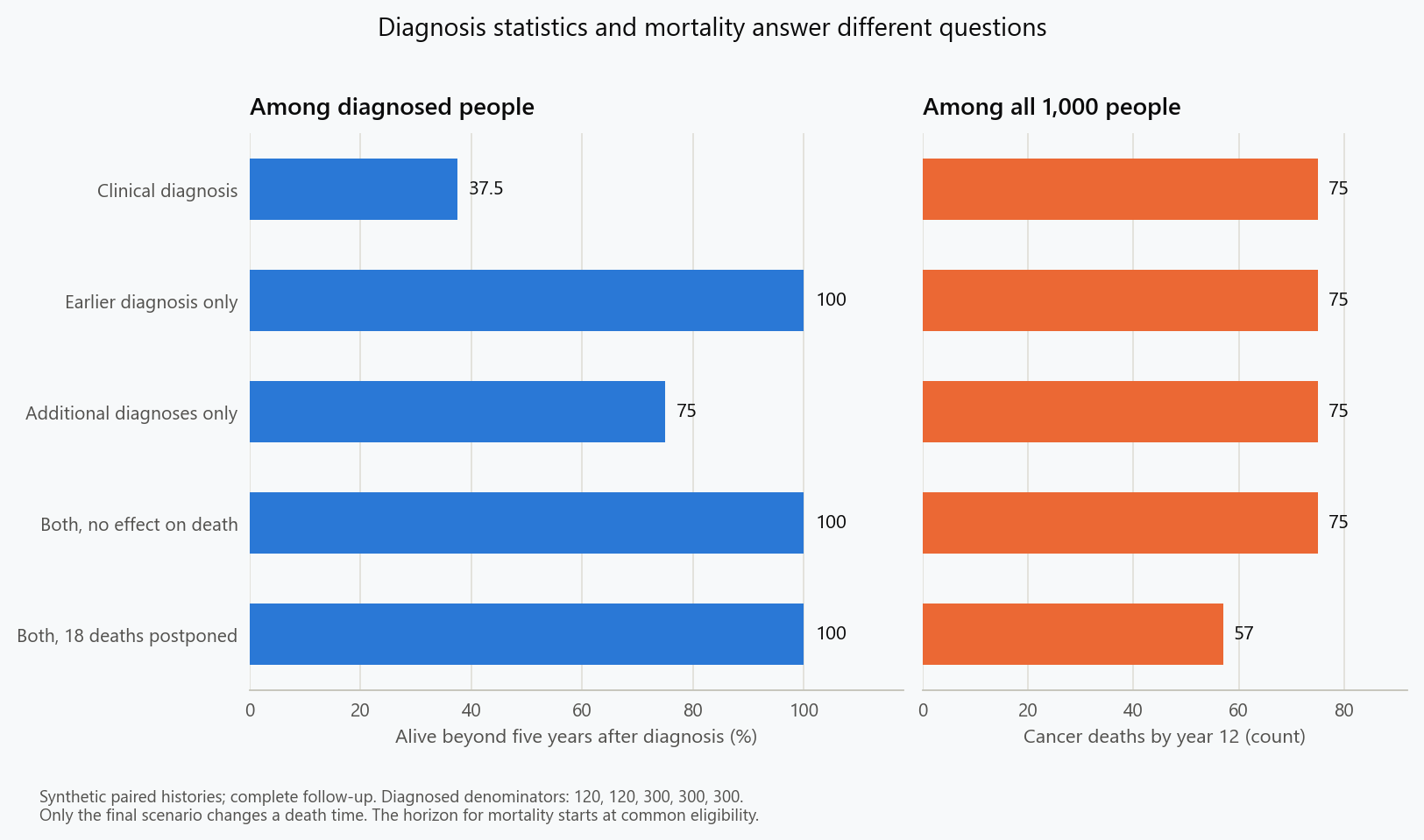
The survival measure is the proportion of diagnosed people alive strictly beyond five years after their own diagnosis. Mortality is measured by year 12 from the common eligibility date, using all 1,000 people. The two quantities consequently have different time origins and different denominators. Complete follow-up makes every calculation a direct count; censoring methods cannot explain any of the discrepancies.
| Scenario | Diagnosed people | Five-year survivors among diagnosed | Five-year survival | Cancer deaths by year 12 | All deaths by year 12 |
|---|---|---|---|---|---|
| Clinical diagnosis | 120 | 45 | 37.5% | 75 | 125 |
| Earlier diagnosis only | 120 | 120 | 100% | 75 | 125 |
| Additional diagnoses only | 300 | 225 | 75% | 75 | 125 |
| Both changes, no effect on death | 300 | 300 | 100% | 75 | 125 |
| Both changes, with 18 deaths postponed | 300 | 300 | 100% | 57 | 107 |
The first four rows preserve every person's death date and cause. Nevertheless, five-year survival takes three different values. Comparing the final two rows gives the reverse result: the five-year statistic is identical, although 18 fewer people have died by year 12. Cancer-death risk falls from 7.5% to 5.7%, and all-cause death risk from 12.5% to 10.7%, over the specified horizon. These differences are attributable to the outcome changes stipulated in the model. They do not arise from changing membership in the eligible population, which remains fixed across all five scenarios.
The final row also shows why a statement about deaths needs a time horizon. All 1,000 people eventually die by year 20 in this construction. A lower death count by year 12 means that deaths have been postponed beyond that horizon, not that death has been abolished. The model specifies an eleven-year extension for the 18 affected people, but a real trial with twelve years of observation could not simply assume their subsequent lifetime histories. Reporting a risk difference at a stated follow-up time and estimating years of life gained are related tasks with different information requirements.
Changing who receives a diagnosis
The additional-diagnoses scenario concerns overdiagnosis: detecting a lesion that meets the disease definition but would not become clinically consequential during the person's remaining lifetime. It is distinct from a false-positive test, in which a positive result is not confirmed as the target disease. Improving analytical specificity does not automatically resolve overdiagnosis, because a correctly identified lesion can still belong to a disease history that would never have caused symptoms. This distinction is explained in the NCI account of length bias and overdiagnosis. The synthetic cohort knows those histories by construction; an actual patient and clinician generally do not.
For the original 120 diagnosed people, 45 survive beyond five years. Adding 180 people who all survive beyond five years changes the calculation to
No member of the original group has acquired a better outcome. The aggregate changes because the group being averaged has changed. It would be inappropriate to interpret the resulting 37.5-percentage-point increase as an effect experienced by an average patient, since there is no fixed patient population behind that contrast. This is a general issue in data analysis whenever an intervention affects whether someone enters the dataset on which its apparent success is evaluated. Restricting a comparison to diagnosed cases conditions on a variable downstream of the detection strategy.
Stage percentages can inherit a related denominator problem. Suppose 30 of the original 120 cases are classified as advanced and all 180 additional diagnoses are classified as early stage. The advanced-stage proportion falls from 25% to 10%, while the number of advanced cases remains 30 per 1,000 eligible people. This particular change reflects dilution, without a reduction in advanced disease. A decline in advanced-case incidence in comparable populations would supply different information, and its relevance to mortality would still require evaluation. The example does not claim that every observed stage shift is dilution; it shows why the number of advanced cases and the population at risk belong beside the percentage.
Why a snapshot favours long detectable histories
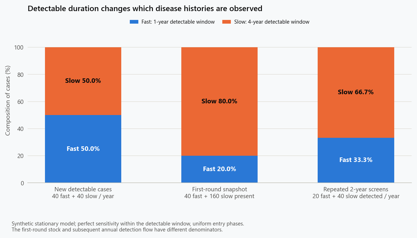
Screening also changes the mixture of progressive disease that is observed. Imagine two disease types entering a preclinical, screen-detectable state at constant rates of 40 cases per year each. The fast type remains detectable without symptoms for one year; the slow type remains in that state for four years. Assume a stationary population, perfect detection during that interval, and no competing death or other exit before the interval ends. At a first examination of a previously unscreened population, the pool of detectable cases includes entrants from one preceding year for the fast type and four preceding years for the slow type.
For a type with entry rate $\lambda_j$ and detectable duration $d_j$, the expected number present is $\lambda_j d_j$. The units make the relationship intelligible: cases per year multiplied by years gives cases. Our two types therefore contribute 40 and 160 detectable cases. Although they make up equal shares of newly entering disease, the slow type accounts for 80% of the snapshot's detections. This distinction between the flow into a state and the stock currently occupying it is central to screening models. The preclinical-to-clinical framework has a long mathematical history, including Zelen and Feinleib's 1969 stochastic treatment.
For several types, the probability that a detected case belongs to type $j$ is
Thus an equal number of incident cases does not imply an equal number of screen-detected cases. This is length-biased sampling: longer intervals have more opportunities to intersect the examination date. If longer detectable intervals are associated with more favourable prognosis, screen-detected cases can have better outcomes even before any benefit from intervention is introduced. That association is a further biological condition, not something proved by the sampling formula. A longer detection window describes an observation opportunity; it does not, by itself, identify a disease's lethality or the effect of treatment.
The same argument extends beyond two fixed durations. Let $D$ be detectable duration among incident cases, with density $f(d)$ and finite positive mean. Under the stationary snapshot assumptions, the duration density among detected cases is
Multiplication by $d$ gives long intervals extra weight, while division by the mean restores a total probability of one. If the second moment is finite, the mean duration among detected cases follows directly:
The selected mean exceeds the incident mean whenever durations vary. For equal incident shares with durations one and four years, the incident mean is 2.5 years and the variance is 2.25 squared years. The detected mean is consequently $2.5+2.25/2.5=3.4$ years. This difference is produced entirely by sampling, with no change to any disease trajectory. If every duration were identical, the variance term would vanish and this source of compositional distortion would disappear. That limiting case is useful because it identifies the heterogeneity that the mechanism requires.
Repeated screening changes the weighting
A prevalence calculation for a first screening round should not be applied unchanged to every subsequent round. Once detected cases have been removed from the undiagnosed pool, later examinations encounter a different population. To make the distinction explicit, suppose screening occurs every $\Delta$ years and new cases enter their detectable state at uniformly distributed phases relative to that schedule. The waiting time $U$ from entry to the next examination is uniform between zero and $\Delta$. With perfect sensitivity, a case with duration $d$ is detected before symptoms if the next examination falls inside its detectable interval. Hence
With examinations two years apart, a one-year window is intercepted with probability one-half, while a four-year window is intercepted with probability one. The expected annual flow of newly detected cases is therefore 20 fast and 40 slow cases. Slow cases now make up two-thirds of detections, compared with 80% at the initial snapshot and 50% among all new detectable cases. These statements concern different sampling processes and are compatible. Cases are counted only at their first detection; the annual flow is a long-run average over screening cycles, not the number seen at every single examination.
This calculation makes the model's limits visible. Real sensitivity may depend on lesion size and time since onset; participation may be irregular; entry rates may change with age; and competing death can truncate the opportunity for detection. False negatives would also make later examinations relevant after a missed first opportunity. More frequent screening changes the mixture sampled under our assumptions, but the formula contains no treatment effect, resource constraint, or harm. It therefore cannot select an optimal interval or establish a mortality benefit. Those decisions require a model and evidence that connect detection to subsequent clinical outcomes.
Returning to a common population and clock
To evaluate whether a screening strategy reduces deaths, eligibility and follow-up should be defined before the strategy can change diagnosis. Let $a$ denote assignment to a specified strategy, and let $T^a$ be the potential time of death from the common entry date under that strategy. An all-cause mortality target at time $t$ is
The probability is defined in the same eligible population for each strategy. A comparison such as $R_1(t)-R_0(t)$ asks how death risk changes under the alternatives over that horizon. For death from the target cancer, let $C^a$ denote cause of death and define the cumulative incidence
In both definitions, people who never receive a cancer diagnosis remain in the population. Their exclusion would discard part of the intervention's effect on diagnostic inclusion and could destroy comparability. Other-cause deaths also remain part of the history. For an actual probability of cancer death by a given time, they are competing events; treating them as ordinary censoring in a Kaplan–Meier complement generally targets a different quantity. The synthetic table avoids that estimation issue by providing every outcome, but a real analysis must handle follow-up and competing risks consistently with its stated target.
Random assignment of eligible people to a screening offer and a defined comparator provides a way to estimate an effect without observing both histories for each person. An intention-to-treat analysis retains people in their assigned groups regardless of subsequent attendance. Its result concerns the effect of that offer under the trial's participation and follow-up conditions. Restricting the comparison to people who complied can reintroduce differences in health, access, or behaviour, because attendance itself was not randomised. Similarly, comparing screen-detected cases with symptom-detected cases cannot inherit the protection of an original random allocation after case selection has changed the groups.
Cancer-specific and all-cause mortality answer complementary questions. The former focuses on the disease that screening is intended to affect but depends on cause-of-death classification. The latter includes fatal harms and avoids assigning a cause, while an effect on one cancer may be small relative to variation in deaths from all other causes. Failure to demonstrate a statistically significant all-cause reduction is therefore not, by itself, proof that a cancer-specific effect is absent. Follow-up duration, uncertainty, treatment after detection, and nonfatal harms also matter. The endpoint should be judged against the claim and the study's ability to estimate it.
None of this makes survival analysis uninformative. Prognosis after a defined diagnosis is a legitimate question, and survival measured from a common randomisation point can evaluate treatments. Population survival trends can also contribute to an assessment of progress when interpreted alongside incidence and mortality. Cho and colleagues' analysis of cancer trends demonstrates why those measures need to be considered together. The methodological objection arises when a change in conditional post-diagnosis survival is presented as sufficient evidence of screening benefit, with the effects of diagnosis timing and selection left unresolved.
A trial that measured a mortality benefit
The National Lung Screening Trial illustrates the stronger comparison. Its 2011 report described 53,454 participants at high risk of lung cancer, randomised to three annual rounds of low-dose computed tomography or chest radiography. Reported lung-cancer mortality was 247 versus 309 deaths per 100,000 person-years, corresponding to a 20.0% relative reduction, with a 95% confidence interval from 6.8% to 26.7%. These are the trial's reported results, not outputs of the synthetic cohort. The comparator was chest radiography, and the participants were a defined high-risk population; neither detail should disappear when the result is communicated. NLST Research Team, 2011.
The inferential advance lies in following randomised groups for deaths rather than judging the strategy by survival among the cancers it detected. The reported figures are mortality rates, using person-time, whereas the synthetic table reports cumulative risks over twelve years. Subtracting the trial's rates gives 62 deaths per 100,000 person-years; it does not directly give 62 deaths prevented per 100,000 people screened. Translating a result into an absolute individual risk requires the corresponding population and follow-up information. This is the same denominator discipline developed in Read the Starting Risk Before the Percentage, now applied to a time-to-event outcome.
Reading an early-detection claim carefully
For a social-media graphic, the first task is to reconstruct the comparison hidden behind the headline. A percentage labelled “survival” needs an origin, a duration, an event definition, and a denominator. Five years after diagnosis, five years after randomisation, and five years after the first positive test describe different measurements. Overall survival and relative survival, which adjusts against expected background survival, are also distinct. Adjustment for background mortality does not automatically undo an earlier starting clock or the inclusion of extra indolent cases. A sophisticated estimator cannot recover comparability simply through its name.
The next task is to identify what observation would discriminate between benefit and the alternative explanations. If a claim reports more early-stage diagnoses, examine advanced-case counts in the full eligible population. If it reports better survival among detected cases, examine mortality from a common entry date and the way comparison groups were formed. If it reports a relative reduction, recover the absolute frequency, time scale, uncertainty, and comparator. For a proposed screening programme, consequences such as additional procedures and treatment of inconsequential disease belong alongside possible benefits. Detection is an intermediate event in that chain of consequences, rather than a complete measure of its value.
The synthetic examples support a precise conclusion: longer survival after diagnosis can arise without longer life, and the same survival percentage can accompany different effects on mortality. They do not determine whether a named test helps a particular population. That requires empirical evidence about a specified strategy, including what happens after detection. Scientific communication becomes more useful when it preserves those boundaries: the starting clock explains what has been measured, the denominator explains whose experience has been counted, and a credible comparison explains which changes can be attributed to the intervention.
Reproducing the calculations
The figure generator and synthetic histories create the same 1,000 identities for each scenario, retaining each person's diagnosis time, death time, and cause. Its dry run prints the complete scenario summaries and the duration-selection calculations without writing figures. No patient dataset, fitted parameter, or random seed is needed: the first model is deterministic, and the second uses exact stationary expectations. From the reproducibility repository, run
1
poetry run python scripts/figures/health/screening_survival.py --dry-run
Omitting the flag regenerates the two figures. The model checks verify that the first four scenarios preserve every death history and that the beneficial scenario changes exactly 18 histories. Separate interval counting checks the snapshot calculation, a grid of entry phases checks repeated-screen detection, and equal-duration and time-unit transformations check the formulas' limits. These checks establish that the published calculations follow the stated assumptions. They cannot establish that an actual disease satisfies those assumptions; that boundary is part of the article's argument.
References
- National Cancer Institute. Crunching Numbers: What Cancer Screening Statistics Really Tell Us. Updated 16 July 2018.
- Zelen M, Feinleib M. On the theory of screening for chronic diseases. Biometrika. 1969;56(3):601–614.
- Cho H, Mariotto AB, Schwartz LM, Luo J, Woloshin S. When Do Changes in Cancer Survival Mean Progress? The Insight From Population Incidence and Mortality. Journal of the National Cancer Institute Monographs. 2014;2014(49):187–197.
- National Lung Screening Trial Research Team. Reduced Lung-Cancer Mortality with Low-Dose Computed Tomographic Screening. New England Journal of Medicine. 2011;365(5):395–409.
Embed interactive plots, widgets, and demos using <figure>, <iframe>, or <div class="interactive-embed"> containers. Ensure each embed includes descriptive captions for accessibility.
How to cite
Use the quick export buttons to save citations for reference managers or copy the formatted text directly.
Diogo Ribeiro (2025). Why Longer Survival After Diagnosis Can Mislead. Faculty of Media Arts and Design, Technical University of Porto. https://diogoribeiro7.github.io/science-communication/why_longer_survival_after_diagnosis_can_mislead/.