Topics
A poll shared on a social network can acquire an authority that appears proportional to its response count. A result based on a million votes seems difficult to question when a conventional survey might interview only a thousand people. The larger number appears to promise both democratic breadth and statistical precision: many people have spoken, so the reported percentage should closely describe what people think. That conclusion contains an unstated step. The people who encountered the question, chose to answer it, and remained in the recorded dataset must somehow stand in for the population named in the headline. Counting more responses does not establish that relationship.
This problem persists even when every response is authentic. There need be no automated account, duplicate submission, purchased vote, or misleading chart. People with different opinions may have different probabilities of following the account, seeing the post, trusting its author, or finding the question worth answering. Those probabilities can alter the composition of the recorded opinions before an analyst calculates a mean. The arithmetic can then be flawless while the inference is inaccurate. The central issue is how observations entered the dataset, together with what can be learned about people who did not enter it.
The following examples use invented populations with known answers. Their purpose is to make selection visible, rather than estimate the quality of a particular platform or polling organisation. Starting from exact counts, we will examine why apparent precision increases, what demographic weighting can repair, and how populations with substantially different opinions can produce identical recorded responses. This approach also preserves an essential distinction: an observation can describe its respondents correctly while failing to describe a larger population. Scientific criticism becomes more useful when it specifies which of those claims the data support.
Archive note: this article is filed under 12 September 2024. It was prepared and source-checked on 19 September 2026; its cited research predates the archive date.
Defining the population before counting its opinions
Suppose the question concerns support for a proposed public policy among all eligible adults in a defined region on a specified date. Let $Y_i=1$ indicate that person $i$ supports the proposal and $Y_i=0$ otherwise. For a population of $N$ people, the target proportion is
Now let $R_i=1$ if that person's answer is recorded and $R_i=0$ if it is absent. The observed response count is $n=\sum_iR_i$, and the respondent proportion is
These are different averages. The first includes everyone in the target population; the second includes only recorded respondents. Calling the second quantity “public support” introduces a claim about the relationship between $R_i$ and $Y_i$. Calling it “support among people who answered this poll” makes a narrower descriptive claim. Neither the platform's number of registered accounts nor the number of impressions automatically supplies the missing denominator, because accounts may not correspond to unique eligible people and an impression need not represent an opportunity to participate on comparable terms.
The target itself must also be stable enough to interpret. A poll of an account's followers can answer a useful question about those followers, provided their membership and recording process are understood. It becomes a different analysis when the caption describes all residents, all patients, or all voters. Similar changes occur when a question about preference is recast as a statement about factual correctness: even a representative measure of what people believe does not establish whether the belief is true. Population inference and evaluation of a scientific proposition require different links between the observations and the conclusion.
A million responses with a known error
Consider a synthetic population of 20 million people. Twelve million support the proposal and eight million do not, so population support is 60%. Suppose 8% of supporters and 2% of other people have their responses recorded. These fractions summarise the entire observation process: access, exposure, participation, and retention. They need not be caused by any single platform feature. To keep the example exact, stipulate the counts below rather than drawing a random sample. Everyone reports their opinion correctly, and no person appears twice.
| Opinion | People in population | Fraction recorded | Recorded responses |
|---|---|---|---|
| Support | 12,000,000 | 8% | 960,000 |
| Do not support | 8,000,000 | 2% | 160,000 |
| Total | 20,000,000 | 5.6% | 1,120,000 |
The poll reports $960{,}000/1{,}120{,}000=6/7$, or approximately 85.714% support. The difference from the target is 25.714 percentage points. Every one of the 1.12 million observations is genuine; the discrepancy results from supporters appearing at four times the rate of other people. The number of responses does not obscure the mechanism once the full table is available. In an actual poll, however, the first two columns are generally unavailable for the opinion being measured. The analyst observes the selected answers and must justify whatever connection is made to the unobserved population.
For a population support proportion $p$, write $r_1$ and $r_0$ for the recorded fractions among supporters and other people. Dividing recorded supporters by all recorded people gives
If both fractions are positive, the corresponding odds satisfy
Selection multiplies population odds by a recording-rate ratio. Here the population odds are $0.6/0.4=1.5$, and the recording ratio is four, giving respondent odds of six and a respondent proportion of $6/7$. This calculation identifies exactly which imbalance produces the error. It also explains why a high overall response count cannot diagnose the problem: the count combines the two recording fractions, whereas the distortion depends on their relative values and on the population's composition.
Increasing reach uniformly does not repair that ratio. If both recording fractions are multiplied by the same positive factor, while remaining no greater than one, the multiplier cancels from the expression for $q$. More people enter the dataset, but the selected proportion remains unchanged. A campaign can therefore gather responses much faster without moving its estimate closer to population support. Targeted recruitment of underrepresented people would change a different part of the mechanism. Whether it succeeds depends on whom it reaches and whether selection remains associated with opinion among those people.
What a shrinking interval is measuring
An analyst who treats the recorded answers as independent Bernoulli observations might report a normal-approximation interval centred on $q$, with half-width
At $q=6/7$ and $n=1{,}120{,}000$, the half-width is approximately 0.0648 percentage points. The resulting interval is approximately 85.649% to 85.779%. Its narrowness reflects the sample-size term in the formula, not evidence that selection has become negligible. Because the synthetic counts were stipulated, this is an illustration of what the naive calculation reports, rather than a valid confidence statement for those fixed counts. In particular, it supplies no justification for attaching 95% coverage to the unknown population proportion.
To separate bias and variance formally, consider a second, explicitly stochastic model: independent draws with replacement from a distribution whose support probability is $q$. If $\widehat q_n$ is the resulting sample proportion, then $\mathbb E[\widehat q_n]=q$ and its variance is $q(1-q)/n$. Its mean squared error when used to estimate the different quantity $p$ is
The variance term decreases as observations accumulate; the squared bias remains. Under this model, the law of large numbers makes the estimate converge to $q$. That is successful convergence for the respondent distribution, with no promise that $q=p$. The independent-draw model is an analytical comparison, not a claim that a viral poll has independent participation. Dependence between respondents could create additional uncertainty, but it is unnecessary for the selection error demonstrated here.
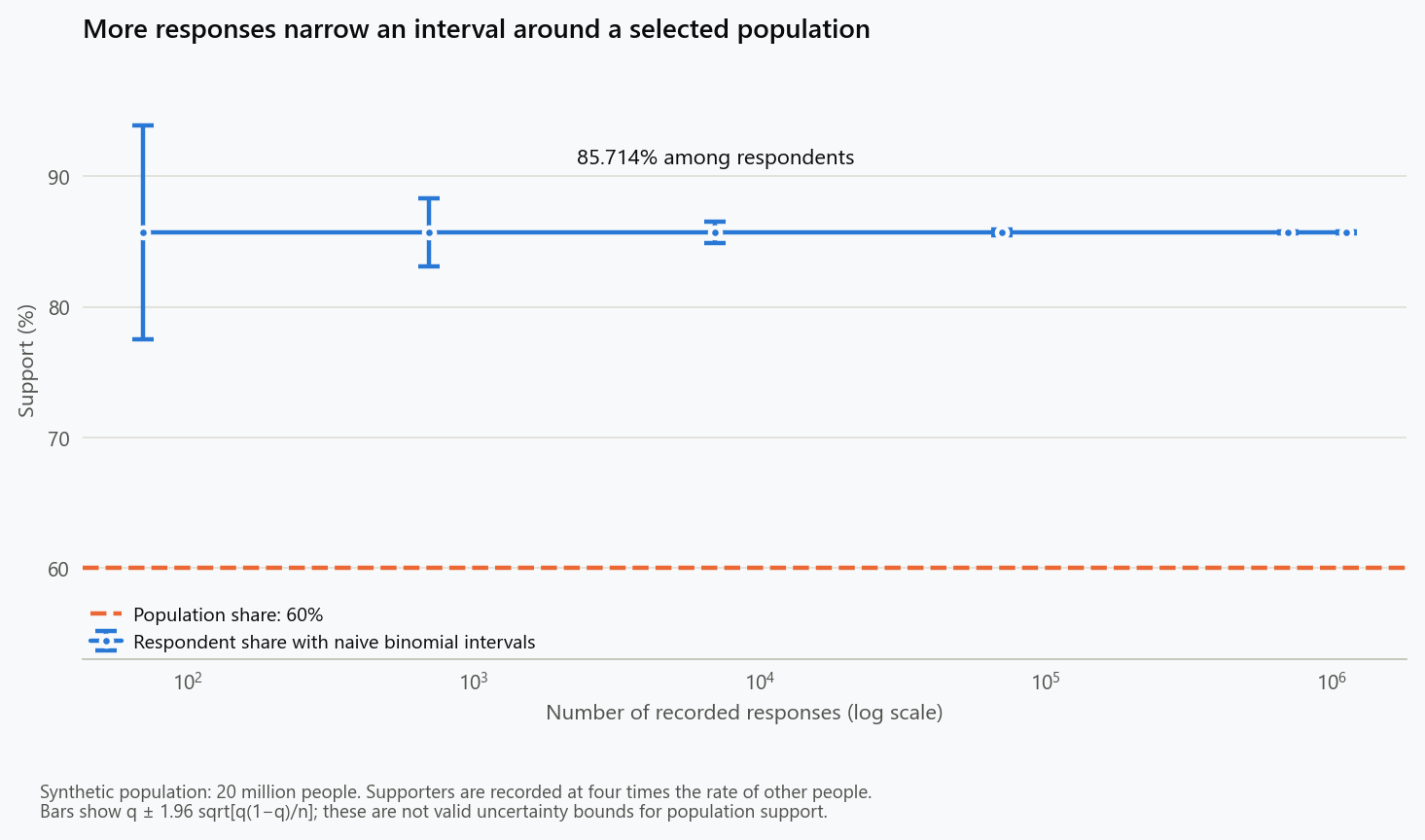
For comparison, an ideal simple random sample of 1,000 people without replacement from this same population has a design standard error of about 1.55 percentage points. Its sample mean is unbiased under the sampling design, and a normal reference half-width is about 3.04 points. Those numbers do not guarantee that one realised sample is accurate, and practical surveys still confront nonresponse and measurement error. They show why a smaller sample with a defensible connection to the population can provide more useful information than a much larger collection with a persistent selection error. The comparison concerns the observation processes, not a preference for small datasets.
An exact covariance account of selection
The error can also be expressed without assigning a probability model to the sampling process. Take means, variances, and covariances across the complete finite population, using divisor $N$. The average of $R$ is the recorded fraction $f=n/N$, and the average of $RY$ is $fq$. Therefore
Since a binary recording indicator has variance $f(1-f)$, writing the covariance as a correlation times two standard deviations yields
for $0<f<1$ and nonconstant $Y$. This is the finite-population error identity central to Xiao-Li Meng's analysis of the big data paradox. It separates the association between recording and outcome, the variability of the outcome, and the fraction of the population observed. It is an identity for a realised dataset, rather than a guarantee that any particular selection mechanism has a given error.
In our table, $f=0.056$, $\sigma_Y=\sqrt{0.6\times0.4}$, and the recording-outcome correlation is approximately 0.128. Multiplying the terms recovers the 0.25714 difference between the two proportions. The correlation uses outcomes for the entire population, including people whose answers are missing from the poll. It cannot generally be computed from respondents alone. Estimating it requires additional information or assumptions; substituting zero because the unobserved association cannot be measured would assume away precisely the issue under investigation.
The identity also prevents an overstatement of the argument. Observing a larger fraction can improve matters, and a complete census with accurate measurements has no selection error for this mean. At a census, $R$ is constant, so the correlation is undefined and the difference should be evaluated directly as zero. At intermediate fractions, the correlation can change as recruitment expands. Sample size, recording fraction, and selection quality should therefore be examined together. A general claim that larger samples must be worse would be as poorly justified as a claim that larger samples must be representative.
When weighting repairs the imbalance
Demographic weighting attempts to use information about the population that is available even when the target opinion is not. Consider a separate population of 100,000 people divided into two observed groups, A and B. Group A contains 40% of the population and has 90% support; group B contains 60% and has 40% support. Overall support is again $0.4\times0.9+0.6\times0.4=0.6$. Initially suppose that 10% of each opinion within A is recorded and 2% of each opinion within B is recorded. Selection differs between groups, while recorded people reproduce the opinion distribution inside each group.
| Group | Population | Population supporters | Recorded supporters | Recorded other people |
|---|---|---|---|---|
| A | 40,000 | 36,000 | 3,600 | 400 |
| B | 60,000 | 24,000 | 480 | 720 |
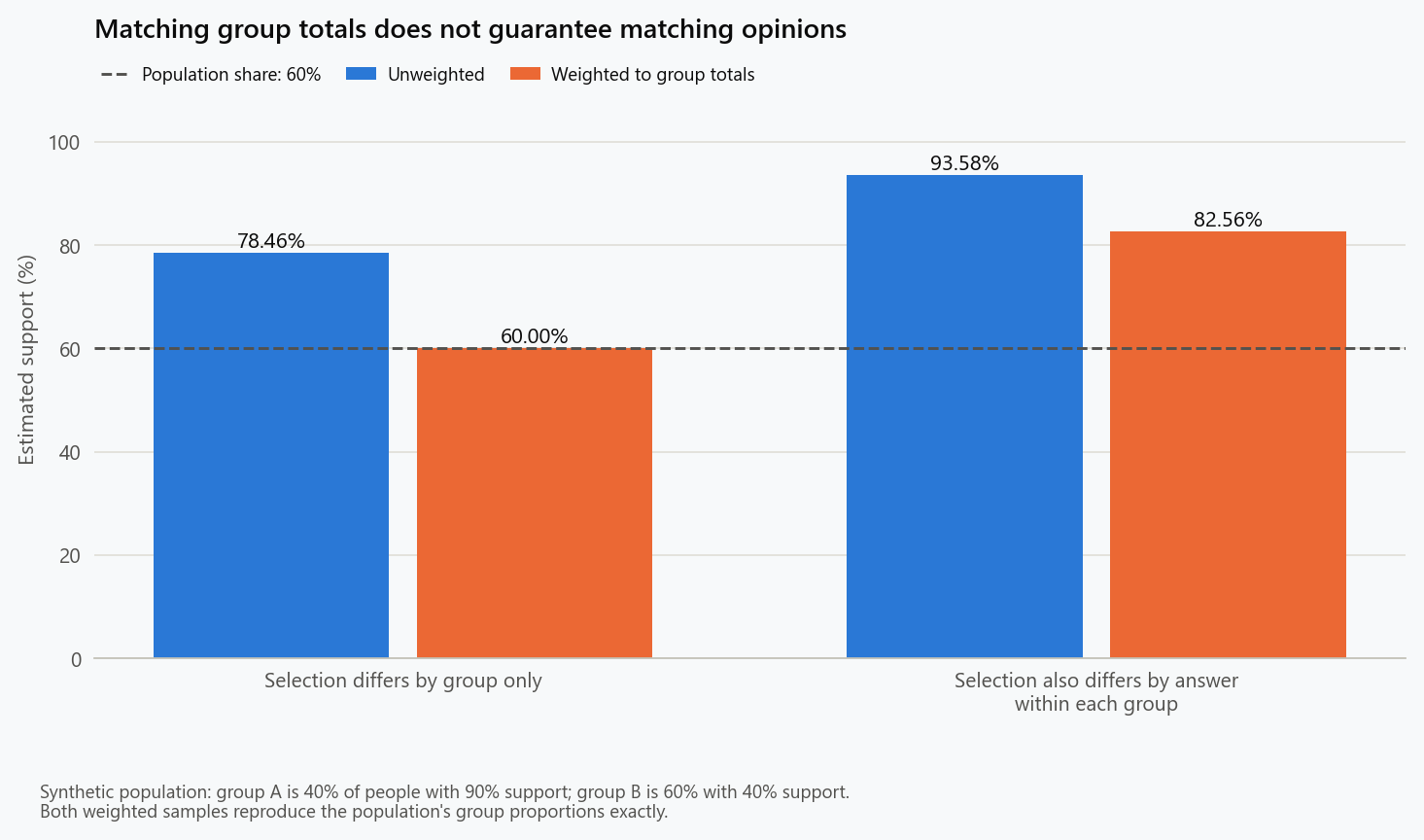
The unweighted estimate is $4{,}080/5{,}200$, approximately 78.46%. Group A is overrepresented and has greater support, so the raw average is too high. Weighting each A response by 10 and each B response by 50 restores the known group totals. Equivalently, poststratification averages the two respondent proportions using population group shares:
Here $W_A=0.4$, $W_B=0.6$, $q_A=0.9$, and $q_B=0.4$, giving exactly 60%. The correction works because the observed variable partitions the selection mechanism in the needed way. Within each group, the observed opinion proportion equals the population opinion proportion. In a stochastic formulation, an assumption such as $Y\perp R\mid G$, combined with adequate coverage of the groups, would justify learning group-level opinion distributions from respondents. Known group totals alone do not establish that assumption.
Now retain the same population and the same numbers of recorded supporters, but divide recorded nonsupporters in each group by four. The recorded counts become 3,600 supporters and 100 other people in A, and 480 supporters and 180 other people in B. The respondent proportions are now $36/37$ and $8/11$. Reweighting still reproduces the population's 40%–60% group composition exactly, but the resulting estimate is
Support remains overstated by about 22.56 percentage points after demographic balance has been achieved. Matching the observed group distribution repaired between-group composition, but the respondent opinions within each group were still distorted. In general, the remaining error is $\sum_gW_g(q_g-p_g)$, where $p_g$ is the population opinion proportion in group $g$. A validation table showing balanced demographics therefore verifies one property of the weighted dataset. It does not verify that the unobserved opinions within those demographic categories have also been represented.
Identical responses can conceal different populations
Return to the original 960,000 recorded supporters and 160,000 recorded nonsupporters in a population of 20 million. Consider three possible worlds. In the first, half the population supports the policy, with recording fractions of 9.6% among supporters and 1.6% among other people. In the second, support is 60% and the fractions are 8% and 2%, as before. In the third, support is 75% and the fractions are 6.4% and 3.2%. Each produces exactly the same observed counts. The response count and reported proportion cannot distinguish them.
| Population support | Supporter recording fraction | Other recording fraction | Recorded supporters | Recorded other people |
|---|---|---|---|---|
| 50% | 9.6% | 1.6% | 960,000 | 160,000 |
| 60% | 8.0% | 2.0% | 960,000 | 160,000 |
| 75% | 6.4% | 3.2% | 960,000 | 160,000 |
This is an identification problem. The available observations are compatible with several values of the target because changes in population opinion can be offset by changes in recording. More precise arithmetic on the same table cannot choose among those worlds. Additional observations or restrictions must enter somewhere: a probability sample, a credible external benchmark, information about recruitment, or an assumption connecting missing answers to observed characteristics. A complex predictive model may encode such restrictions, but its complexity does not make them empirically established.
Even without a selection model, knowing the population size gives a simple bound. Write $u$ for support among unrecorded people. Then
Since $0\leq u\leq1$, the possible population proportion lies between $fq$ and $fq+1-f$. For the original table, this range is 4.8% to 99.2%. These extreme completions assume that every unrecorded person gives the same answer; they are not assertions that either extreme is plausible. They show what the counts alone establish under the stated information. Substantive knowledge can narrow the range, but that knowledge should be identified explicitly rather than disguised as a consequence of having many responses.
Turning an untestable certainty into a sensitivity analysis
A more informative analysis can ask how conclusions change across specified selection assumptions. Let $\lambda=r_1/r_0$ be the ratio of recording fractions. Solving the earlier equation for population support gives
For the observed proportion $q=6/7$, this simplifies to $p=6/(6+\lambda)$. Equal recording fractions, $\lambda=1$, imply 85.714% population support. Ratios of two, four, and six imply 75%, 60%, and 50%, respectively. Thus a belief that supporters are between twice and six times as likely to be recorded would imply population support between 50% and 75% in this model. Each endpoint is compatible with the observed recording fraction; implied recording probabilities remain within zero and one.
That range is conditional on the analyst's selection assumptions. It is not a 95% confidence interval, a posterior credible interval, or an estimate that the true ratio lies between two and six. A defensible application would explain the evidence used to choose those values, perhaps through a validation sample or recruitment study, and would also account for uncertainty in the observed proportion where a stochastic model is appropriate. The benefit of sensitivity analysis is that it locates the disagreement in an explicit parameter. Readers can see which assumptions preserve a conclusion and which alter it materially.
In the synthetic example, knowing the correct ratio of four recovers the population proportion exactly. In an actual survey, the opinions needed to estimate that ratio are precisely those that are missing. Asking respondents whether they are representative would not measure the recording behaviour of nonrespondents. Nor would collecting another large sample through the same channel necessarily supply independent information about the mechanism. A useful follow-up changes what is learned about missing people, rather than merely enlarging the set of people already easy to observe.
What resampling and empirical comparisons add
Bootstrapping the observed poll does not automatically solve this problem. Resampling its recorded responses reproduces a dataset with a support fraction near $q$, so bootstrap estimates concentrate around that selected proportion. The procedure can approximate variation under an empirical respondent distribution while remaining silent about how that distribution differs from the target population. Resampling methods are valuable when they match the inferential problem; they cannot manufacture information about people absent from the sampling frame. A selection-adjusted bootstrap would need a justified adjustment model, with its assumptions carried into the uncertainty analysis.
The distinction between an online data-collection mode and a probability-based recruitment design is also consequential. A survey completed on the internet can recruit from randomly selected addresses, whereas a link distributed to willing visitors has a different selection process. AAPOR's 2010 report on online panels distinguishes these recruitment approaches and examines the limits of applying conventional sampling-error claims to opt-in data. Random initial recruitment still leaves practical problems of participation and retention. The methodological question is how a study addresses each stage, rather than whether its questionnaire appears on a screen.
An empirical comparison illustrates why those distinctions deserve measurement. In a study published in 2023, Pew Research Center applied a common questionnaire and weighting scheme to three probability-based online panels and three opt-in samples, with 29,937 interviews collected in 2021. Across 28 benchmark variables, average absolute error was 2.6 percentage points for the probability-based panels and 5.8 for the opt-in samples. These are study-specific averages, not universal error allowances. The benchmark sources were themselves imperfect, and the comparison examined total error rather than isolating our synthetic selection mechanism. Mercer and Lau, 2023.
Those results support evaluating methods against independent information while resisting a categorical conclusion that one design label guarantees accuracy on every variable. A population can be represented adequately for one outcome and poorly for another, because recording may be associated with those outcomes differently. The same reasoning explains why matching age and region does not automatically validate estimates of trust, engagement, or a specialised belief. What matters is whether the design and adjustment address the relationships relevant to the quantity being estimated.
Reading the claim attached to the number
For a viral poll, the first task is to reconstruct the population named by the claim and the route by which people entered the dataset. A count of completed answers should be accompanied by an account of eligibility, recruitment, missingness, and any removal of responses. The next task is to establish what weighting used and what it assumes about people within the weighted groups. Finally, the interval around the reported percentage needs an interpretation: which repeated process or probability model does it describe, and does that model include selection uncertainty? A familiar interval formula cannot answer those questions on behalf of the study.
Large collections can still document what participants reported, reveal differences within a defined user community, generate hypotheses, and support models whose assumptions can be examined against external data. The restriction concerns generalisation beyond what those observations establish. In the worked examples, more responses made the respondent proportion increasingly precise, demographic weighting repaired only the imbalances it addressed, and identical response counts remained compatible with different populations. A useful account of evidence makes those distinctions visible before the headline converts participation into representation.
Reproducing the examples
The calculation and figure generator uses exact integer counts for the finite populations and ordinary arithmetic for the formulas. It does not download survey records or simulate opinions. Six recording levels retain the same population while preserving the four-to-one recording ratio; separate tables reproduce both weighting scenarios and the three observationally equivalent worlds. The dry run prints all values without creating figures, from the reproducibility repository:
1
poetry run python scripts/figures/statistics/poll_selection.py --dry-run
Omitting the flag regenerates the two figures. The independent model checks reconstruct covariance from individual records, enumerate every simple random sample in a small population, expand weighted responses, and examine every completion of a small set of missing answers. Equal-recording and census cases check the boundaries of the argument. These checks verify that the numerical claims follow from the stipulated populations and mechanisms; empirical claims about a real poll require evidence about its own recruitment and response processes.
References
- Meng X-L. Statistical paradises and paradoxes in big data (I): Law of large populations, big data paradox, and the 2016 US presidential election. The Annals of Applied Statistics. 2018;12(2):685–726. Author-hosted full text.
- Baker R, Blumberg SJ, Brick JM, et al. Research Synthesis: AAPOR Report on Online Panels. Public Opinion Quarterly. 2010;74(4):711–781. AAPOR-hosted full text.
- Mercer A, Lau A. Comparing Two Types of Online Survey Samples. Pew Research Center. 7 September 2023.
Embed interactive plots, widgets, and demos using <figure>, <iframe>, or <div class="interactive-embed"> containers. Ensure each embed includes descriptive captions for accessibility.
How to cite
Use the quick export buttons to save citations for reference managers or copy the formatted text directly.
Diogo Ribeiro (2024). Why a Million Responses Can Still Give the Wrong Answer. Faculty of Media Arts and Design, Technical University of Porto. https://diogoribeiro7.github.io/science-communication/why_a_million_responses_can_still_give_the_wrong_answer/.