Topics
Claims that thought creates external reality often appeal to a recognisable description of quantum mechanics: particles behave differently when they are observed. The description then acquires an extra meaning. Observation becomes conscious attention, a change in experimental statistics becomes a decision made by a mind, and the observer's intention is presented as a force capable of selecting the desired result. These are separate propositions. An experiment showing that a detector changes interference does not, by itself, establish that awareness caused the change, that a person selected an outcome, or that the same mechanism explains events outside the apparatus.
Quantum measurement deserves a more careful explanation than either mystical certainty or dismissive reassurance. Its mathematical predictions are precise, and experiments constrain them, but the interpretation of a measurement remains a serious subject. We can distinguish those levels by calculating what an apparatus does before asking what the calculation means philosophically. The relevant variables include the prepared state, relative phases, interactions with a detector, and which outcomes are combined or separated in the analysis. A proposal about consciousness must add something to that account: a specified change in the predicted observations, together with evidence that distinguishes it from ordinary physical effects.
The model below is deliberately small enough to examine completely. It represents two coherent paths and a two-state physical marker, uses the usual Born rule for probabilities, and assumes ideal operations without detector losses or background counts. Its figures are calculated predictions, not measurements from a laboratory. Within that setting, the model explains reduced interference, partial information about a path, and the complementary patterns of a quantum eraser. It also identifies the limits of the explanation, including why a reduced density matrix does not settle the measurement problem.
Archive note: this article is filed under 23 January 2025. It was prepared and source-checked on 19 September 2026; all cited research predates the archive date.
Beginning with amplitudes and an apparatus
Consider an interferometer with two path alternatives, represented by orthogonal states $\lvert0\rangle$ and $\lvert1\rangle$. A ket is a vector describing a quantum state; the labels identify alternatives in a chosen basis. Suppose the preparation gives the paths equal amplitudes, with a controllable relative phase $\phi$. Before the paths are recombined, write the state as
An ideal recombination followed by detection in two output ports is equivalent, with a suitable phase convention, to measuring in the basis $\lvert+\rangle=(\lvert0\rangle+\lvert1\rangle)/\sqrt2$ and $\lvert-\rangle=(\lvert0\rangle-\lvert1\rangle)/\sqrt2$. The probability of the positive output is the squared magnitude of its amplitude:
The other probability is $P(-)=1-P(+)$. At zero phase, every ideal detection goes to the positive port; at phase $\pi$, every detection goes to the negative port. Between those settings, the probabilities vary continuously. Interference is the phase-dependent cross term produced when amplitudes are added before their squared magnitude is taken. It would be absent if the two alternatives were treated from the outset as a classical mixture with equal probabilities and no relative coherence.
This calculation concerns repeated preparations and outcome frequencies. It does not say that an individual person can choose which detector clicks. Changing an optical path length or another physical phase control changes the probability distribution by changing the apparatus. Wishing for a different click has not been assigned an operation in the model. Nor does the observation of an interference curve, by itself, establish every specifically quantum feature of a source: classical waves can also interfere. The present question concerns how path information and quantum correlations alter the predictions for the stipulated preparation.
A physical record changes the joint state
Introduce a marker whose state can become correlated with the path. After an ideal interaction, let path 0 be associated with $\lvert d_0\rangle$ and path 1 with $\lvert d_1\rangle$. The joint state is
The marker could represent an internal atomic state, a polarisation degree of freedom, or another physical system. Its role is specified by the interaction and by the distinguishability of its possible states. No reading of a display is required to write this joint state. If the marker states are identical, the marker contains no information that distinguishes the two paths. If they are orthogonal, an appropriate marker measurement can distinguish the alternatives perfectly. Intermediate overlaps encode partial distinguishability.
Use the explicit family $\lvert d_0\rangle=(1,0)$ and $\lvert d_1\rangle=(\gamma,\sqrt{1-\gamma^2})$, where $0\leq\gamma\leq1$. Their overlap is the real number $\gamma$. A general overlap can be complex, with its phase affecting the fringe position; restricting it to a nonnegative real value keeps the present calculation focused on contrast. If marker results are not included in the path analysis, predictions use the reduced path state obtained by tracing over the marker:
Tracing over the marker means summing over a complete set of marker alternatives when predicting measurements on the path alone. It does not mean that the experimenter has mentally destroyed the marker or forced it to acquire a value. The off-diagonal entries retain the phase information accessible to the path interference experiment, scaled by the marker overlap. Applying the same output measurement as before gives
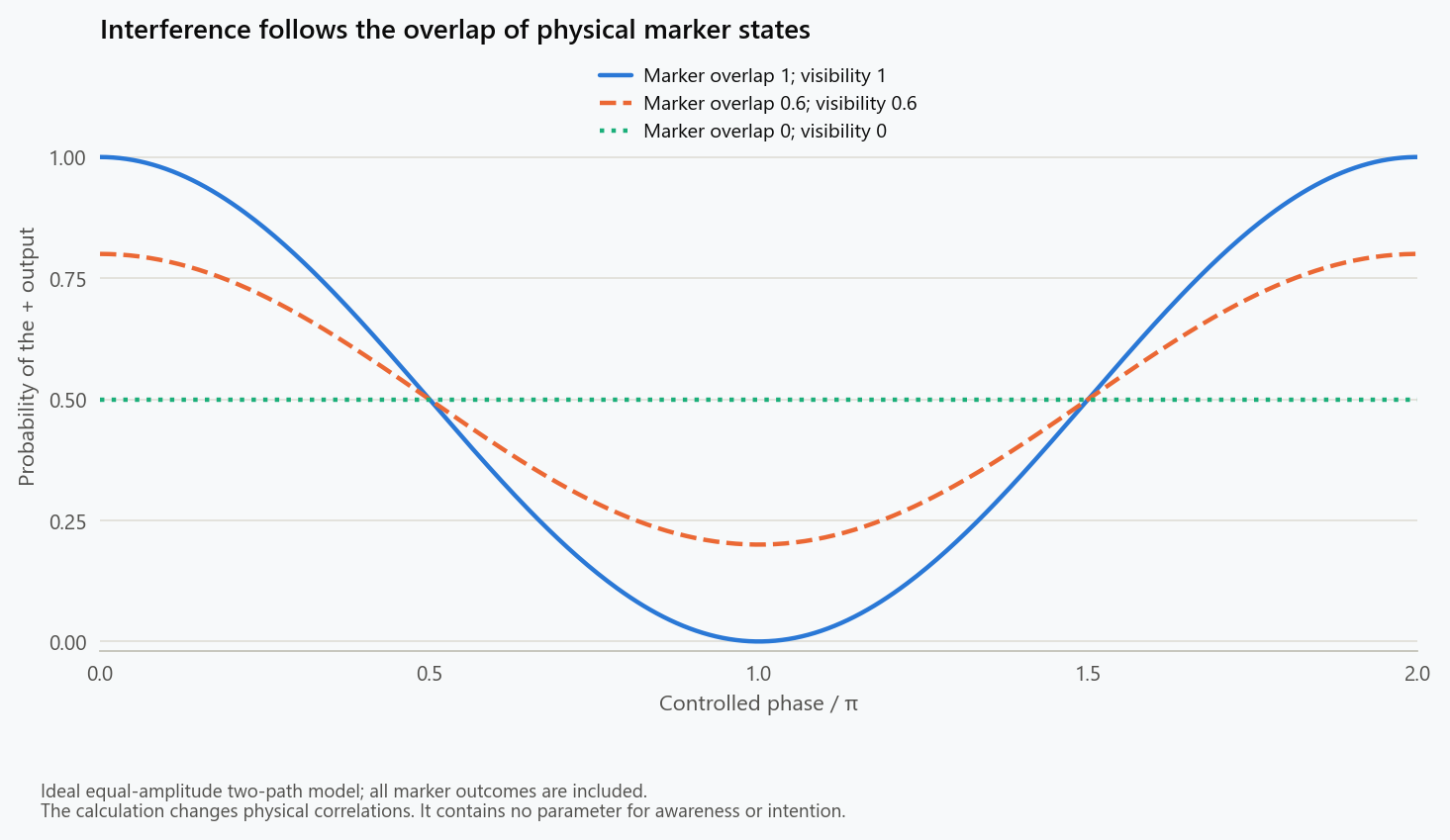
Thus a physical correlation changes the distribution even when nobody reads a path record. At $\gamma=0$, the unsorted outputs are equally probable for every phase. At $\gamma=1$, the original interference is recovered. The reduced state's purity is $\operatorname{Tr}(\rho_{\mathrm{path}}^2)=(1+\gamma^2)/2$, although the stipulated joint state remains pure. Mixedness of a subsystem can therefore reflect correlations with another system. Treating that reduced mixture as proof that the joint system secretly occupied one definite path would add an interpretation that the partial trace does not establish.
The same prediction from four amplitudes
The reduced density matrix is convenient, but the interference result can also be checked directly. There are four combinations of two paths and two marker basis states. In the chosen marker basis, the prepared joint amplitudes form the matrix
Rows label paths and columns label marker states. To obtain the positive output, add the two path amplitudes in each column and divide by $\sqrt2$. The amplitudes for positive output together with marker basis result 0 or 1 are consequently
When marker results are unreported, these are distinct orthogonal marker alternatives, so their probabilities are summed. Adding their amplitudes together would describe a different, coherent projection on the marker, rather than ignoring its outcome. The required calculation is
This gives a concrete meaning to the phrase “information is available in principle”. The joint state contains physically distinguishable alternatives, and the appropriate probability calculation respects them whether or not a result is displayed. With orthogonal path markers, the two positive-output contributions each have probability one-quarter and their sum has no phase dependence. With identical markers, both path amplitudes contribute to the same marker alternative and can interfere fully. It is the arrangement of amplitudes and distinguishable records that changes; a person's decision to inspect the final data does not appear in the calculation.
The same distinction explains why ignoring a record and measuring it in a complementary basis are different operations. Ignoring the marker sums over its alternatives. A complementary measurement combines marker amplitudes before assigning outcomes and creates a new set of joint probabilities. If those new outcomes are subsequently ignored as well, the same path marginal returns. Keeping track of the order in which amplitudes are combined, squared, and summed prevents the everyday word “observation” from concealing mathematically different procedures.
Quantifying the information–interference trade-off
For a phase scan, define fringe visibility by the difference between maximum and minimum detection probability divided by their sum. In this model,
The amount of available path information can be given a separate operational definition. Imagine being supplied with either marker state with equal prior probability and having to guess which state was supplied. This discrimination problem quantifies how reliably the marker distinguishes the alternatives; it does not require assuming a classical trajectory in every coherent experimental run. For these two pure states, the best success probability is
To see the structure, let $\rho_0$ and $\rho_1$ be the marker density matrices and define $\Delta=\rho_0-\rho_1$. If one measurement outcome, represented by an operator $E$ with $0\leq E\leq I$, is assigned the guess “0”, the success probability is $[1+\operatorname{Tr}(E\Delta)]/2$. In our real two-state family, $\Delta$ has eigenvalues $\pm\sqrt{1-\gamma^2}$. Selecting its positive eigenspace maximises the success probability. The distinguishability $D$ is therefore derived from an attainable measurement, rather than introduced as a psychological measure of how certain an observer feels.
Consequently $V^2+D^2=1$ for this ideal family. This is a saturating case of the visibility–distinguishability relation developed in Englert's 1996 analysis. The equality depends on the assumptions used here, including pure marker states and the specified balanced preparation; more general situations need not saturate the appropriate inequality. “Information” in this calculation concerns physical state discrimination. It should not be silently replaced with awareness, semantic understanding, or a person's confidence about an outcome.
| Marker overlap | Visibility | Distinguishability | Best marker-based guess | Range of positive-output probability |
|---|---|---|---|---|
| 1.0 | 1.0 | 0.0 | 50% | 0 to 1 |
| 0.6 | 0.6 | 0.8 | 90% | 0.2 to 0.8 |
| 0.0 | 0.0 | 1.0 | 100% | 0.5 to 0.5 |
The middle row is useful because it avoids a misleading all-or-nothing account. A marker that permits 90% optimal discrimination still allows visible interference with contrast 0.6. At phase zero, the positive output has probability 0.8; at phase $\pi$, it has probability 0.2. These are compatible consequences of the same joint state. Neither quantity reports how much a person has looked at the experiment, and perfect discrimination and full visibility are not simultaneously available under these assumptions.
Turning those probabilities into a measurement requires repeated trials and a sampling model. For 10,000 independent ideal trials at phase zero with $\gamma=0.6$, the expected positive-output count is 8,000 and its binomial standard deviation is 40. A finite run need not produce exactly 8,000 clicks. At a single fixed phase, an observed fraction also cannot separately identify visibility and phase, because both enter through $\gamma\cos\phi$. A controlled phase scan supplies information that one output percentage does not. The plotted curves therefore represent a calibrated theoretical relationship, not an assertion that experimental data lie exactly on a line.
Real inference must also account for departures from the ideal setup, such as background counts, phase drift, unequal efficiencies, and imperfect preparation. A change in fitted contrast needs to be assessed against those mechanisms and its statistical uncertainty before being assigned a new cause. Repeatedly obtaining an approximately flat distribution is evidence about accessible interference under the tested conditions; it does not, without further controls, reveal which physical interaction or preparation history produced that distribution. The phase-averaging example below makes this limitation explicit even with unlimited local data.
Records can spread without being read
A laboratory marker is only one possible recipient of correlations. Suppose the two paths become associated with environment states $\lvert E_0\rangle$ and $\lvert E_1\rangle$. If, conditionally on the path, those environment states factor into independent components, their overlap is the product of the component overlaps:
For an illustrative real overlap of 0.95 per component, the resulting visibility is $0.95^m$: approximately 0.358 after 20 components and 0.00592 after 100. These are dimensionless model values, not estimates of a decoherence time in a particular material. The calculation shows how many individually modest correlations can make local interference extremely small. It assumes conditional product states; an actual environment can have correlations and dynamics that require a more complete treatment.
The physical basis of environment-induced decoherence is developed in Zurek's review. For our purpose, the important implication is that interactions can distribute records into degrees of freedom that are never consciously inspected. Closing a display or declining to read a result does not reverse those interactions. Recovering coherence requires suitable physical control of the relevant correlations, if such control is possible; a change in personal knowledge is not automatically the required operation.
Deleting a classical file should likewise not be confused with a quantum eraser. A macroscopic record can have been copied into electronics, scattered light, heat, or other environmental degrees of freedom. Overwriting one storage location does not restore the coherent joint state that existed before those correlations spread. The controlled eraser calculation below concerns a marker that remains available for a complementary quantum measurement. Its assumptions are much stronger than the ordinary-language statement that somebody forgot which path occurred.
What a quantum eraser restores
Take perfectly distinguishable markers, $\lvert d_0\rangle=\lvert0\rangle$ and $\lvert d_1\rangle=\lvert1\rangle$. The joint state is entangled and the unsorted path outputs each have probability one-half. Instead of measuring the marker in its path-distinguishing basis, measure it in the complementary basis
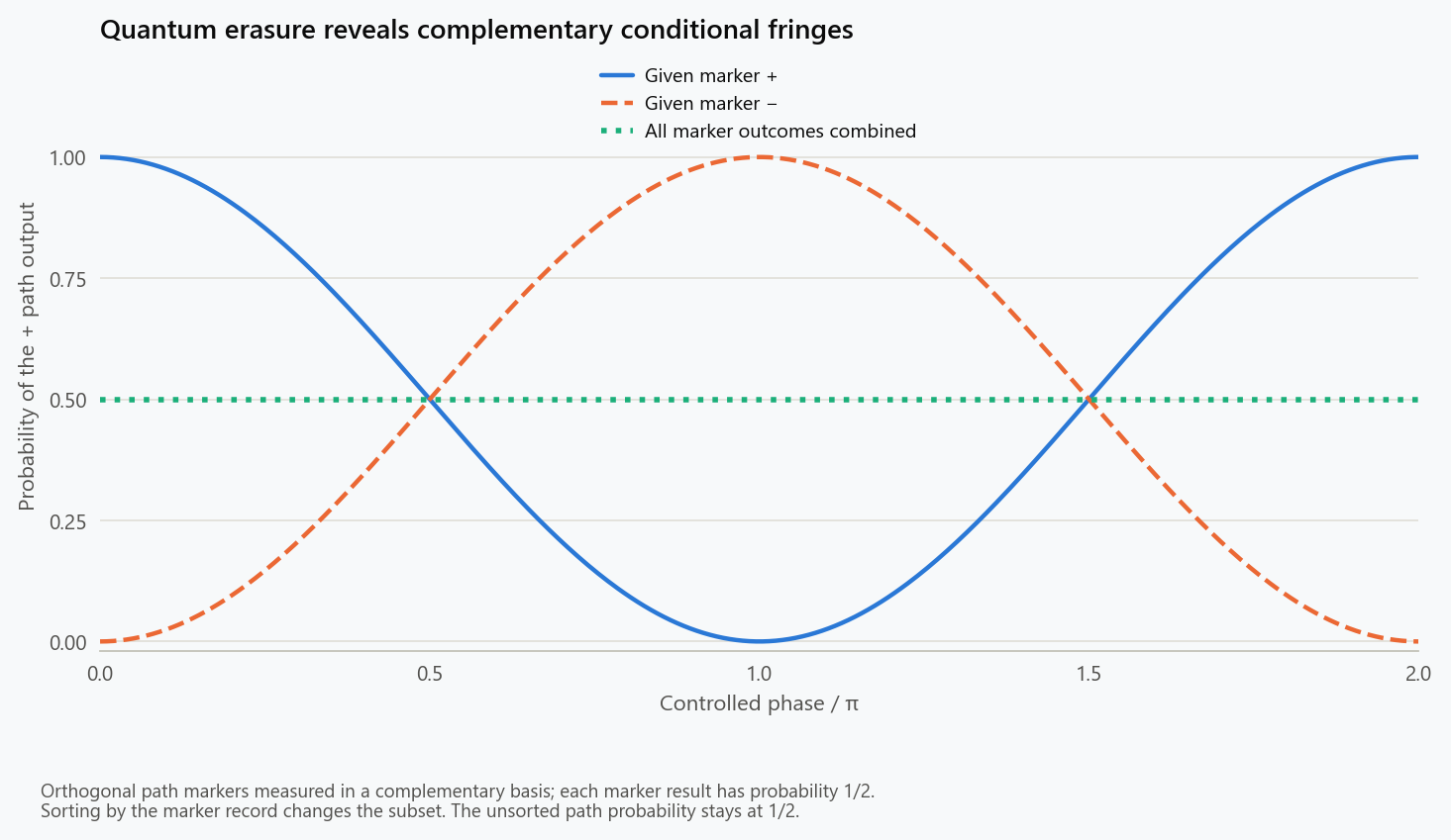
Conditioning on marker result $m_+$ leaves a path state proportional to $\lvert0\rangle+e^{i\phi}\lvert1\rangle$; conditioning on $m_-$ leaves one proportional to $\lvert0\rangle-e^{i\phi}\lvert1\rangle$. Each marker result occurs with probability one-half. The corresponding conditional probabilities are
Each subset has full visibility, but the two fringes are shifted by $\pi$. One subset reaches a maximum exactly where the other reaches a minimum. Combining them with their correct weights returns the original marginal probability:
The following table gives expected counts for 10,000 ideal repetitions at each phase. Each row describes a separate ensemble prepared at that phase; these are theoretical expectations, not observed counts. The two central columns partition the positive-output events by marker result. There are another 5,000 expected negative-output events in every row, distributed between marker results according to the complementary joint probabilities.
| Phase | Positive output and marker + | Positive output and marker − | All positive outputs | Positive fraction within marker + subset |
|---|---|---|---|---|
| 0 | 5,000 | 0 | 5,000 | 100% |
| π/2 | 2,500 | 2,500 | 5,000 | 50% |
| π | 0 | 5,000 | 5,000 | 0% |
The changing final column is a conditional frequency. Its denominator is the 5,000 expected events with marker result $m_+$, not all 10,000 runs. Showing that column while omitting its complementary subset can create the impression that interference reappeared throughout the path data. The complete table establishes something more specific: correlations permit a partition into complementary fringes, while the unsorted output distribution remains unchanged. The distinction follows directly from the joint probabilities and does not depend on whether the sorting is done by a person or by software.
Delayed sorting does not supply a signal to the past
The marker measurement can be performed after the path result has been registered, provided the relevant physical correlations are maintained. The later marker result determines which subset an earlier path event belongs to when the records are compared. That temporal order does not turn the conditional probability into a changed marginal probability. In this model, the unsorted path data remain evenly divided between the outputs. Someone with access only to those data cannot infer which marker basis was chosen elsewhere, much less extract a message sent by selecting that basis.
The underlying identity is general for local projective measurements. Let $\Pi_a$ denote a path-outcome projector and $Q_b$ a marker-outcome projector, with $\sum_bQ_b=I$. For a joint state $\rho$, summing the joint probabilities gives
The marker basis disappears from the marginal after its outcomes are summed. Also, the local projectors $\Pi_a\otimes I$ and $I\otimes Q_b$ commute, so their order does not alter the joint probabilities in this ideal description. These statements concern operations on separate subsystems without subsequent interactions that feed one system's result into the other. Conditioning on a selected marker outcome changes a subset, and feedback can change later outcomes, but neither should be confused with changing an already recorded unsorted distribution by a freely chosen remote basis.
The distinction is relevant to the experiment reported by Kim and colleagues in 2000. Their entangled-photon apparatus recorded delayed joint detections, and the eraser coincidence patterns had opposite phases. The two-port calculation here is an idealisation, not a reconstruction of their spatial optics or detector efficiencies. It reproduces the distinction needed to read such results: correlations appear when records are compared, and complementary conditional patterns must not be substituted for the unsorted data. The experiment does not require an account in which a conscious decision rewrites a previously recorded event.
A missing fringe does not uniquely identify its cause
Even the inference from reduced visibility to path marking needs suitable controls. Consider an alternative preparation with no marker. On each run, prepare a pure path state with relative phase either $\phi+\alpha$ or $\phi-\alpha$, choosing the two options with equal probability. The average phase factor is
Choosing $\alpha=\arccos\gamma$ produces exactly the same reduced path density matrix as the path-marker model. At $\gamma=0.6$, both constructions predict a positive-output range from 0.2 to 0.8. More strongly, they give the same probabilities for every measurement on the path subsystem alone, because those probabilities depend on the same density matrix. A local fringe curve therefore cannot distinguish the entangled preparation from this random-phase ensemble. Measurements involving a controlled marker or a phase record can supply additional information.
This is an identifiability limit, rather than a defect in quantum theory. Different preparation histories can produce the same local statistical state. If an experiment changes when someone approaches the apparatus, plausible physical changes in phase, coupling, alignment, or data selection must be examined before attributing the difference to consciousness. The model does not assert that all losses of visibility are phase noise, any more than it asserts that all of them are path marking. It specifies two mechanisms with identical local predictions and thereby demonstrates what a local measurement cannot decide on its own.
What experiments establish and interpretation leaves open
Physical path records are experimentally meaningful. In their 1998 atom-interferometer study, Dürr, Nonn, and Rempe reported disappearance of interference when which-way information was stored in internal atomic states. They found that the momentum disturbance in their setup was too small to explain that disappearance and attributed it to correlations between the marker and atomic motion. This supports treating the record as part of the quantum system. It also cautions against a universal explanation in which every loss of interference is simply a large mechanical kick delivered by a measuring device.
The calculation above nevertheless assumes the Born rule, the state description, and the operational rules for measurements. It does not derive why one particular outcome is experienced in an individual run. Decoherence explains suppression of local interference and the distribution of correlations into an environment; by itself, that calculation does not select a unique interpretation of quantum mechanics. In particular, obtaining a diagonal reduced density matrix does not prove that the global pure state has become an ordinary ignorance mixture of already definite outcomes. Keeping that distinction explicit is part of explaining the physics accurately.
An unresolved interpretive question also does not establish a particular alternative. To infer that intention controls outcomes, one would need a theory specifying how intention changes the state, dynamics, or probability rule, together with observations that distinguish that change from the standard account. The ordinary experimenter already influences an experiment through physical actions: preparing a source, rotating a polariser, setting a phase, or choosing a measurement basis. Those interventions have mathematical descriptions. Relabelling them as evidence that thought alone selects external events adds a causal claim that the observations have not isolated.
A careful reading of an “observer effect” claim therefore begins with the operation being performed and the distribution being reported. The operation might create a path record, randomise a phase, measure a marker in a new basis, or sort already recorded coincidences. The displayed quantity might be a marginal frequency over all events or a conditional frequency within a selected subset. In the worked examples, those distinctions fully determine the predicted curves without a variable for awareness. Quantum measurement remains conceptually demanding, but that difficulty is a reason to preserve the mathematical distinctions rather than replace them with a claim about the power of intention.
Reproducing the calculations
The calculation and figure generator represents the joint state as four complex amplitudes. It computes probabilities by projecting those amplitudes onto path and marker measurement bases, traces over the marker for local predictions, and reproduces the tables and two figures. The core arithmetic uses the Python standard library; Matplotlib is required only to regenerate figures. Print the model values without writing images with
1
poetry run python scripts/figures/physics/quantum_observer.py --dry-run
The independent model checks compare amplitude projections with the analytic interference formula, search measurement orientations to verify optimal discrimination, and check that arbitrary marker bases leave the path marginal unchanged. They also compare explicit local projectors in both orders, reconstruct the phase-averaged counterexample, and expand small environment tensor products. These checks establish consistency within the ideal model; they do not replace calibration, noise modelling, and empirical controls in an actual experiment.
References
- Englert B-G. Fringe Visibility and Which-Way Information: An Inequality. Physical Review Letters. 1996;77:2154–2157.
- Dürr S, Nonn T, Rempe G. Origin of quantum-mechanical complementarity probed by a ‘which-way’ experiment in an atom interferometer. Nature. 1998;395:33–37.
- Kim Y-H, Yu R, Kulik SP, Shih Y, Scully MO. Delayed “Choice” Quantum Eraser. Physical Review Letters. 2000;84:1–5. Author preprint.
- Zurek WH. Decoherence, einselection, and the quantum origins of the classical. Reviews of Modern Physics. 2003;75:715–775.
Embed interactive plots, widgets, and demos using <figure>, <iframe>, or <div class="interactive-embed"> containers. Ensure each embed includes descriptive captions for accessibility.
How to cite
Use the quick export buttons to save citations for reference managers or copy the formatted text directly.
Diogo Ribeiro (2025). Quantum Measurement Does Not Establish That Thoughts Create Reality. Faculty of Media Arts and Design, Technical University of Porto. https://diogoribeiro7.github.io/science-communication/quantum_measurement_and_the_observer_myth/.