Rolling Windows in Signal Processing

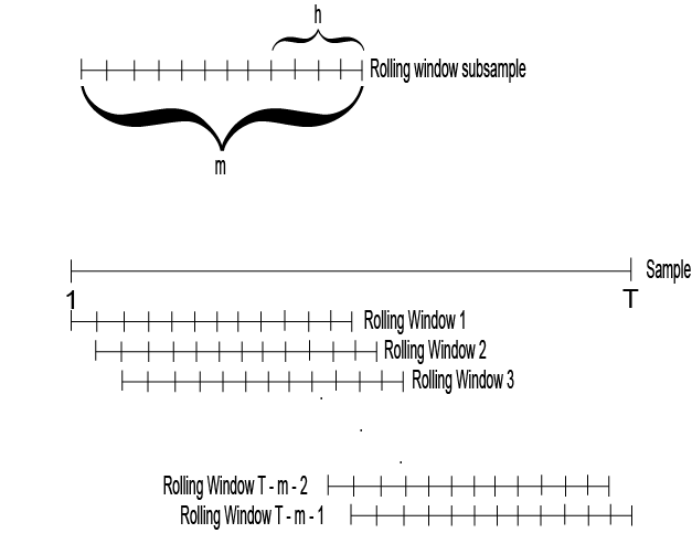
A rolling window is not merely a programming convenience. It defines a local observation operator on a signal, and its width, alignment, stride, taper, and overlap determine which temporal structures are visible and which are averaged away. In predictive maintenance this is especially important because the same sensor stream can support very different tasks: smoothing, local feature extraction, transient detection, spectral analysis, or prediction of a future failure state.

1. Window definition and alignment

For a discrete signal x[t], a trailing window of length n ending at time t is

A centered window uses observations on both sides of t, while a leading window uses future observations. That distinction is critical. Centered smoothing may be appropriate for retrospective signal analysis, but it causes leakage if the resulting feature is used for real-time prediction.

With stride s, window endpoints occur at

Large overlap gives smoother temporal resolution but creates strongly dependent feature rows. Treating heavily overlapping windows as independent observations can make validation results look much more precise than they really are.

2. Window length determines the time scale

A short window responds quickly to local changes but produces noisy estimates. A long window reduces variance but can average across transients or regime changes.

The correct width should be tied to the physical process. For vibration data it may correspond to several shaft rotations. For temperature degradation it may correspond to minutes or hours. Choosing a window only because it performs well on a test set risks overfitting the validation design.

3. Local feature extraction

For a window w_t with n samples, common features include

and root-mean-square amplitude

Other features may include peak-to-peak range, crest factor, kurtosis, zero-crossing rate, band power, spectral centroid, or domain-specific harmonics.

Feature choice should follow the failure mechanism. A bearing defect that creates impulsive high-frequency vibration calls for different features from a slow thermal drift.

4. Smoothing is filtering

A moving average of width n is a finite impulse response filter with coefficients

Its output is

This filter suppresses some high-frequency variation, but it also has a specific frequency response. It is therefore inaccurate to describe smoothing as simply removing noise while preserving signal. Whether variation is noise or useful information depends on the spectrum of the process and the downstream task.

A trailing moving average also introduces delay. A centered moving average can remove that phase delay in retrospective analysis, but it cannot be used causally in real time without future data.

5. Savitzky-Golay smoothing

Savitzky-Golay filtering fits a low-degree polynomial within each local window and evaluates the fitted polynomial at a chosen location. For a centered window with offsets i=-k,…,k, the local coefficients solve

The resulting filter can preserve polynomial shape and local peak structure better than a simple moving average. It does not universally preserve every peak or transient. Its behavior depends on window length, polynomial order, edge handling, and signal structure.

6. Peak detection requires a noise model

A local threshold such as

can be useful when mean and scale evolve slowly. But this is not a generic peak detector. If the local distribution is heavy-tailed, autocorrelated, or contaminated by previous peaks, the threshold may be poorly calibrated.

Peak detection should also distinguish amplitude from prominence, width, refractory distance, and persistence. In rotating machinery, the timing and frequency of repeated peaks may be more informative than one large sample.

7. STFT and window functions

The short-time Fourier transform analyzes local spectra by multiplying the signal by a window function g and computing a Fourier transform at successive time positions:

The window function is not the same thing as the rolling data slice. A rectangular window corresponds to abruptly truncating the segment. Tapers such as Hann or Hamming windows reduce spectral leakage by down-weighting samples near the boundaries.

There is a time-frequency trade-off. Long windows improve frequency resolution but blur temporal changes. Short windows localize transients better but spread energy across frequency bins.

8. Overlap does not create new independent information

Suppose windows of length 256 are extracted every 16 samples. Adjacent windows then share 240 samples. Their feature vectors can be extremely similar.

If those overlapping windows are randomly split across training and test sets, nearly identical signal segments can appear on both sides. This is a serious leakage mechanism.

For predictive maintenance, validation should usually split at a higher level such as machine, run, operating episode, or chronological block.

9. Predictive-maintenance labels need temporal discipline

Assume a failure occurs at time T and we want to predict whether failure will occur within horizon h. A label might be

Every feature for Y_t must be computable from information available no later than t. Centered windows, post-maintenance data, future normalization statistics, or features computed across the complete run all leak information from the future.

This is one reason windowing should be designed together with the prediction target rather than added later as feature engineering.

10. A typed Python implementation

1
2
3
4
5
6
7
8
9
10
11
12
13
14
15
16
17
18
19
20
21
22
23
24
25
26
27
28
29
30
31
32
33
34
35
36
37
38
39
40
41
42
43
44
45
46
47
48
49
50
51
52
53
from __future__ import annotations

from dataclasses import dataclass

import numpy as np
import pandas as pd
from numpy.typing import NDArray


@dataclass(frozen=True)
class WindowConfig:
    window_size: int
    stride: int

    def __post_init__(self) -> None:
        if self.window_size <= 1:
            raise ValueError("window_size must be greater than 1")
        if self.stride <= 0:
            raise ValueError("stride must be positive")


def extract_features(
    signal: NDArray[np.float64],
    config: WindowConfig,
) -> pd.DataFrame:
    """Extract trailing-window features from a one-dimensional signal."""
    if signal.ndim != 1:
        raise ValueError("signal must be one-dimensional")
    if signal.size < config.window_size:
        raise ValueError("signal is shorter than window_size")

    rows: list[dict[str, float | int]] = []

    for start in range(
        0,
        signal.size - config.window_size + 1,
        config.stride,
    ):
        stop = start + config.window_size
        window = signal[start:stop]

        rows.append(
            {
                "start": start,
                "stop": stop,
                "mean": float(np.mean(window)),
                "std": float(np.std(window, ddof=1)),
                "rms": float(np.sqrt(np.mean(window**2))),
                "ptp": float(np.ptp(window)),
            }
        )

    return pd.DataFrame(rows)

The function deliberately returns window boundaries. Those indices are useful when joining features back to event times and checking that labels are aligned without leakage.

11. STFT example

1
2
3
4
5
6
7
8
9
10
11
12
13
14
15
16
17
18
19
20
21
22
23
24
25
26
27
28
29
from __future__ import annotations

import numpy as np
from numpy.typing import NDArray
from scipy.signal import stft


def compute_stft(
    signal: NDArray[np.float64],
    sampling_rate_hz: float,
    nperseg: int = 256,
    noverlap: int = 128,
) -> tuple[NDArray[np.float64], NDArray[np.float64], NDArray[np.complex128]]:
    """Compute a Hann-window STFT with validated segment parameters."""
    if signal.ndim != 1:
        raise ValueError("signal must be one-dimensional")
    if sampling_rate_hz <= 0:
        raise ValueError("sampling_rate_hz must be positive")
    if not 0 <= noverlap < nperseg:
        raise ValueError("noverlap must satisfy 0 <= noverlap < nperseg")

    frequencies, times, spectrum = stft(
        signal,
        fs=sampling_rate_hz,
        window="hann",
        nperseg=nperseg,
        noverlap=noverlap,
    )
    return frequencies, times, spectrum

12. Window features are estimators, not facts

A rolling mean, variance, RMS value, or spectral estimate is itself uncertain. Short windows can produce highly variable features, especially under autocorrelation. When such features are fed into a downstream model, that estimation noise becomes part of the learning problem.

This matters when comparing machines with different sampling rates or missingness patterns. Two rows with the same nominal window duration may contain different effective information.

Conclusion

Rolling windows are useful because many signals are locally simpler than they are globally. But every window encodes assumptions about locality, stationarity, information availability, and resolution.

For predictive maintenance, the main questions are not merely which summary functions to compute. They are:

• what physical time scale the window represents
• whether the window is causal at prediction time
• how much adjacent windows overlap
• whether validation separates dependent windows
• whether the chosen features correspond to the failure mechanism
• whether spectral tapering and resolution are appropriate

Treating these choices as part of the statistical model produces more reliable signal features and more credible maintenance predictions.

References

• Oppenheim, A. V., & Schafer, R. W. Discrete-Time Signal Processing.
• Stoica, P., & Moses, R. L. Spectral Analysis of Signals.
• Savitzky, A., & Golay, M. J. E. (1964). Smoothing and Differentiation of Data by Simplified Least Squares Procedures.
• Harris, F. J. (1978). On the Use of Windows for Harmonic Analysis with the Discrete Fourier Transform.