Understanding Markov Chain Monte Carlo (MCMC)

Markov Chain Monte Carlo (MCMC) is a powerful and widely-used class of algorithms designed to sample from probability distributions, especially when direct analytic computation becomes challenging. It has found applications in various domains, particularly in Bayesian statistics, physics, machine learning, and complex probabilistic models. This article explores the foundational concepts behind MCMC, how it works, different MCMC algorithms, and its importance in modern statistical and numerical methods.

What is Markov Chain Monte Carlo?

At its core, Markov Chain Monte Carlo is a family of algorithms that relies on Markov chains to sample from a target probability distribution. The target distribution is typically one that is difficult to sample from directly due to its high-dimensional nature or the complexity of its mathematical form. MCMC methods are designed to approximate this distribution over time by generating a sequence of dependent samples, which, in the long run, tend to represent the target distribution more accurately.

Markov Chains

A Markov chain is a sequence of random variables where the distribution of each variable depends only on the value of the previous one, a property known as the Markov property. More formally, a Markov chain is a sequence of random variables $X_1, X_2, \ldots$ where the conditional probability of $X_{n+1}$ given the entire history up to $X_n$ depends only on $X_n$:

This property simplifies the modeling of the chain, as only the current state influences the next, making computations and approximations manageable.

Monte Carlo Methods

Monte Carlo methods are a class of algorithms that rely on random sampling to estimate numerical quantities, typically integrals. In problems involving high-dimensional spaces, directly calculating integrals or probabilities is often impossible. Monte Carlo methods allow for numerical approximations through repeated random sampling.

Monte Carlo estimation often uses independent draws when direct sampling is available, but Monte Carlo is broader than independent sampling. High dimensionality does not make ordinary Monte Carlo automatically infeasible in the same exponential way as tensor-product quadrature; the difficulty depends on the target distribution and proposal mechanism.

Combining the Two: MCMC

Markov Chain Monte Carlo methods combine the principles of Markov chains and Monte Carlo techniques to produce correlated samples from a target distribution. Unlike traditional Monte Carlo methods where samples are independent, the samples in MCMC are autocorrelated, meaning each sample is dependent on the previous one.

The key idea behind MCMC is to construct a Markov chain such that its stationary distribution (also called the equilibrium distribution) is the target distribution. If the transition kernel has the target distribution as stationary and the chain is irreducible, aperiodic, and sufficiently well behaved, ergodic averages converge to target expectations. Stationarity alone is not enough to guarantee useful sampling from an arbitrary starting point.

The Curse of Dimensionality

One challenge both Monte Carlo methods and MCMC face is the curse of dimensionality. As the number of dimensions increases, the volume of the space grows exponentially. In high-dimensional spaces, regions of high probability can become tiny relative to the overall space, making it hard for random samples to effectively explore these regions.

MCMC addresses this problem better than traditional Monte Carlo methods by focusing on constructing Markov chains that spend more time in regions of high probability, but even MCMC is not immune to the difficulties posed by high-dimensional spaces. Strategies such as tuning the step size of the walk or using more advanced algorithms have been developed to mitigate these challenges.

Applications of MCMC

Markov Chain Monte Carlo methods are highly versatile and find applications in many fields, especially in situations where probability distributions are too complex to handle analytically. Below are some of the key applications:

Bayesian Inference

One of the primary uses of MCMC methods is in Bayesian statistics. In Bayesian inference, we are interested in calculating the posterior distribution of model parameters given observed data. This often involves multi-dimensional integrals that are analytically intractable. MCMC allows us to numerically approximate these integrals by sampling from the posterior distribution.

Bayesian inference often requires the computation of moments, credible intervals, and other summary statistics from the posterior. MCMC makes this feasible, even in models with many parameters or hierarchical structures, where exact computation would be impossible.

Multi-dimensional Integrals

In many scientific and engineering applications, we are required to calculate high-dimensional integrals, such as:

When the dimensionality of $x$ is large, traditional numerical integration techniques become computationally expensive or even infeasible. MCMC provides an efficient way to approximate these integrals by sampling from the distribution defined by $f(x)$ and then averaging over the samples.

Rare Event Sampling

MCMC methods are also valuable in rare event sampling, where the goal is to sample from regions of the probability space that correspond to low-probability, high-impact events. These events are important in fields like reliability engineering, finance, and risk analysis. In these cases, MCMC methods gradually explore the rare failure regions by generating samples that concentrate on the areas of interest, even when these regions are hard to find in a high-dimensional space.

Hierarchical Models

Hierarchical or multi-level models are common in many fields, including medicine, psychology, and econometrics. These models involve parameters at multiple levels of abstraction, each of which may depend on others. The resulting posterior distribution of parameters is often too complex to compute directly.

MCMC makes it possible to fit large hierarchical models by drawing samples from the posterior distribution, allowing for the estimation of the effects at each level of the model. This has made MCMC an indispensable tool in applied statistics.

Key MCMC Algorithms

Several algorithms exist under the umbrella of MCMC. The most common ones include the Metropolis-Hastings algorithm and Gibbs sampling. Each has its own strengths and is suitable for different types of problems.

Metropolis-Hastings Algorithm

The Metropolis-Hastings algorithm is one of the most widely used MCMC methods. It works by constructing a Markov chain through a proposal mechanism. Given the current state of the chain, the algorithm proposes a new state, and the move is accepted or rejected based on the probability of the new state relative to the current state.

Steps of the Metropolis-Hastings Algorithm

1. Start with an initial state $X_0$.
2. Propose a new state $X'$ based on a proposal distribution $q(X' | X_n)$.
3. Compute the acceptance probability:

1. Accept the proposed state with probability $\alpha$. If accepted, set $X_{n+1} = X'$, otherwise, keep the current state: $X_{n+1} = X_n$.
2. Repeat the process to generate the desired number of samples.

The algorithm relies on a proposal distribution, which can be chosen based on the problem at hand. Common choices include Gaussian distributions centered at the current state. The Metropolis algorithm is a special case of the Metropolis-Hastings algorithm where the proposal distribution is symmetric, i.e., $q(X' | X) = q(X | X')$.

Gibbs Sampling

Gibbs sampling is another popular MCMC algorithm, particularly useful when the target distribution has a conditional structure. Instead of proposing a new state globally, Gibbs sampling breaks the problem into components and samples each component conditionally, given the others.

Steps of Gibbs Sampling

1. Initialize all components $X_1, X_2, \ldots, X_n$ of the target distribution.
2. Sample $X_1$ from its conditional distribution, $P(X_1 | X_2, X_3, \ldots, X_n)$.
3. Sample $X_2$ from $P(X_2 | X_1, X_3, \ldots, X_n)$, and so on.
4. Cycle through all components repeatedly to generate samples.

Gibbs sampling is particularly well-suited for models where the conditional distributions are easy to sample from, even if the joint distribution is not. One common application is in Bayesian networks or other graphical models.

Random Walk Monte Carlo

The random walk Monte Carlo method is another form of MCMC, in which the steps taken in the chain are based on a random walk. The new position is proposed as a small perturbation of the current position, and this process is repeated to explore the space.

Unlike independent random samples in traditional Monte Carlo integration, random walk samples are autocorrelated, meaning that each sample is dependent on the previous one. Autocorrelation reduces effective sample size. It is not an efficiency advantage over independent target draws; independent target samples would usually be preferable if they were available. MCMC is useful precisely because such direct sampling is often unavailable.

Convergence and Mixing

A key aspect of any MCMC method is how quickly the Markov chain converges to the target distribution. There is no observable moment at which a finite chain can be certified as having “reached” stationarity. Diagnostics assess mixing and between-chain consistency, but they cannot prove convergence from finite output. However, this does not happen immediately, and a poorly constructed Markov chain may take a long time to converge.

The concept of mixing describes how well the chain explores the target distribution. A well-mixing chain quickly visits all regions of the probability space, whereas a poorly mixing chain may get stuck in certain regions and fail to represent the distribution accurately. The rate of convergence and mixing depends on factors such as the proposal mechanism, step size, and dimensionality of the problem.

Diagnosing Convergence

To ensure the accuracy of MCMC methods, it is important to diagnose whether the chain has converged to the target distribution. Several diagnostic techniques exist, including:

• Trace plots: A plot of the values of the chain over time can indicate whether the chain has stabilized around a particular region.
• Autocorrelation: High autocorrelation between successive samples can indicate poor mixing.
• Rank-normalized split-$\hat R$: compares within- and between-chain variation across multiple chains. Values close to 1 are necessary but not sufficient evidence of good mixing. Effective sample size and trace behavior should be examined as well.

Challenges and Improvements

Despite its widespread use and success, MCMC methods are not without their challenges. One of the primary difficulties is the aforementioned curse of dimensionality. As the number of dimensions increases, the Markov chain may struggle to find and remain in regions of high probability.

Improving Efficiency

Several strategies have been developed to improve the efficiency of MCMC methods. These include:

• Adaptive MCMC: In adaptive MCMC, the proposal mechanism is adjusted dynamically based on the behavior of the chain, improving convergence rates.
• Hamiltonian Monte Carlo (HMC): HMC introduces a physics-based approach to MCMC, using concepts from Hamiltonian mechanics to propose new states. This leads to more efficient exploration of the probability space, especially in high-dimensional problems.

Conclusion

Markov Chain Monte Carlo (MCMC) has revolutionized the way we approach complex probabilistic problems. By constructing Markov chains that approximate the target distribution, MCMC allows for the sampling of highly complex, high-dimensional distributions that are otherwise analytically intractable. With applications ranging from Bayesian inference to rare event sampling, MCMC has become an indispensable tool in both theoretical and applied statistics.

Understanding the underlying principles of MCMC and how different algorithms like Metropolis-Hastings and Gibbs sampling operate is crucial for applying these methods effectively. As MCMC continues to evolve with improvements such as adaptive methods and Hamiltonian Monte Carlo, it remains at the forefront of modern statistical computation.

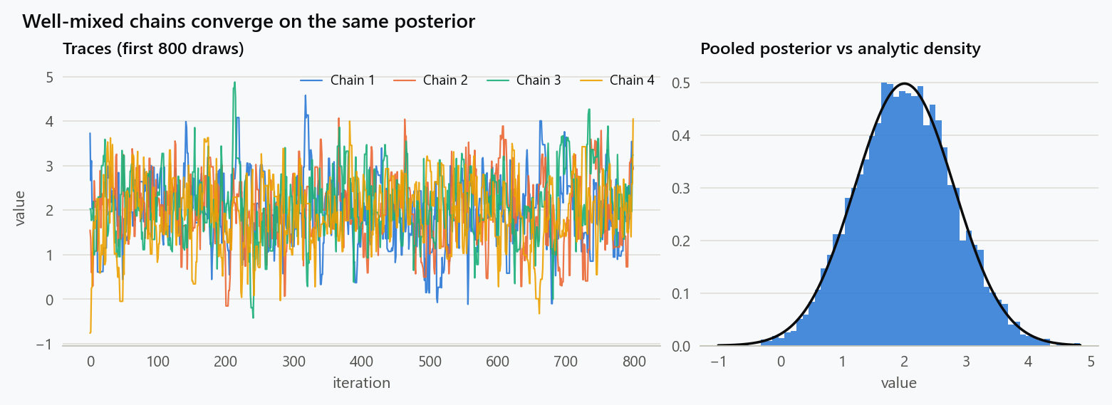
The figure generator in the blog-reproducibility repository reproduces this article's figure; run it with --dry-run to print the numbers behind the figure without writing an image.

Appendix: Python Implementation of the Metropolis-Hastings Algorithm

Below is a simple implementation of the Metropolis-Hastings (MH) algorithm using only base Python and numpy. The goal is to generate samples from a target probability distribution using the MH algorithm. For simplicity, we use a standard normal distribution as our target distribution.

Prerequisites

To run this implementation, you will need the following Python packages:

• numpy (for numerical computations)

You can install numpy by running:

1
pip install numpy

Code Implementation

1
2
3
4
5
6
7
8
9
10
11
12
13
14
15
16
17
18
19
20
21
22
23
24
25
26
27
28
29
30
31
32
33
34
35
36
37
38
39
40
41
42
43
44
45
46
47
48
49
50
51
52
53
54
55
56
57
58
59
60
61
62
63
64
65
66
67
68
69
70
71
72
73
74
75
76
77
78
79
80
import numpy as np

def target_distribution(x):
    """
    Target distribution we want to sample from.
    In this example, it's a standard normal distribution.

Parameters:
    - x: float, the point at which to evaluate the probability density function.

Returns:
    - float, the probability density at point x.
    """
    return np.exp(-0.5 * x ** 2)  # Standard normal distribution (Gaussian)

def proposal_distribution(x, step_size=1.0):
    """
    Proposal distribution to generate a new candidate state.
    We use a symmetric normal distribution centered at the current state.

Parameters:
    - x: float, the current state.
    - step_size: float, the standard deviation of the proposal distribution.

Returns:
    - float, the new candidate state.
    """
    return np.random.normal(loc=x, scale=step_size)

def metropolis_hastings(target_dist, proposal_dist, initial_state, num_samples, step_size=1.0):
    """
    Metropolis-Hastings algorithm to sample from the target distribution.

Parameters:
    - target_dist: function, the target probability distribution.
    - proposal_dist: function, the proposal distribution to generate new states.
    - initial_state: float, the starting point of the Markov chain.
    - num_samples: int, the number of samples to generate.
    - step_size: float, the standard deviation of the proposal distribution.

Returns:
    - samples: numpy array, the generated samples from the target distribution.
    """
    samples = np.zeros(num_samples)
    current_state = initial_state
    samples[0] = current_state

for i in range(1, num_samples):
        # Propose a new state from the proposal distribution
        proposed_state = proposal_dist(current_state, step_size)

# Compute the acceptance probability
        acceptance_ratio = min(
            1.0,
            target_dist(proposed_state)
            / target_dist(current_state),
        )

# Accept or reject the proposed state
        if np.random.rand() < acceptance_ratio:
            current_state = proposed_state  # Accept the new state

samples[i] = current_state  # Store the current state

return samples

# Set parameters
initial_state = 0.0  # Start at x = 0
num_samples = 10000  # Number of samples to generate
step_size = 1.0  # Standard deviation of the proposal distribution

# Run the Metropolis-Hastings algorithm
samples = metropolis_hastings(target_distribution, proposal_distribution, initial_state, num_samples, step_size)

# Summary statistics
mean_estimate = np.mean(samples)
std_estimate = np.std(samples)

print(f"Mean estimate of the samples: {mean_estimate}")
print(f"Standard deviation estimate of the samples: {std_estimate}")

Explanation of the Code

Target Distribution

The target_distribution function defines the probability distribution we wish to sample from. In this example, it represents the standard normal distribution. The probability density function (PDF) of a standard normal is proportional to:

This defines the likelihood of a given value $x$ occurring under the normal distribution.

Proposal Distribution

The proposal_distribution function generates new candidate states based on the current state. In this case, it uses a normal distribution centered around the current state with a tunable step_size. This ensures that the proposed state is "close" to the current state, which is critical for efficient exploration of the target distribution.

Metropolis-Hastings Function

The metropolis_hastings function is the core of the algorithm. It generates a specified number of samples from the target distribution using the Metropolis-Hastings (MH) algorithm. Below is an explanation of how it works:

1. Markov Chain Initialization: The chain starts at an initial state, given by initial_state.
2. State Proposal: A new state is proposed using the proposal_distribution. This state is based on the current state and is generated using a random normal distribution.
3. Acceptance Ratio: The acceptance ratio is calculated as the ratio of the target distribution evaluated at the proposed state to that evaluated at the current state. Mathematically:

This ratio helps determine whether the new state should be accepted based on how much more likely the proposed state is compared to the current one.

1. State Acceptance or Rejection: A random number between 0 and 1 is generated. If this number is less than the acceptance ratio $\alpha$, the new state is accepted. Otherwise, the current state is retained.

2. Sampling Process: The process repeats for a predefined number of samples, and each accepted state is stored in an array to represent the distribution being sampled.

Parameters

In the example implementation, the parameters are set as follows:

• The Markov chain begins at $x = 0$ (initial state).
• The number of samples generated is set to 10,000 (num_samples = 10000).
• The proposal distribution's step size is set to 1.0 (step_size = 1.0), which determines how large the random steps between states are.

These parameters can be modified to better suit other target distributions or exploration strategies.

Output

After running the algorithm, the mean and standard deviation of the sampled values are printed to compare them with the theoretical values for the standard normal distribution (mean 0, standard deviation 1). The estimates should be close to the actual values for a sufficiently large number of samples.

Sample Output

When the algorithm is executed, the following output might be produced:

1
2
Mean estimate of the samples: 0.007
Standard deviation estimate of the samples: 0.996

This output is close to the true mean of 0 and the standard deviation of 1, as expected for a standard normal distribution.

Plotting the Results

You can use matplotlib to visualize the results and verify that the samples follow the target distribution. Below is a Python script that plots a histogram of the generated samples and overlays the true standard normal distribution for comparison:

1
2
3
4
5
6
7
8
9
10
11
12
13
14
15
import matplotlib.pyplot as plt
import numpy as np

# Plot a histogram of the generated samples
plt.hist(samples, bins=50, density=True, alpha=0.6, color='b', label='MCMC Samples')

# Overlay the true standard normal distribution for comparison
x = np.linspace(-4, 4, 1000)
plt.plot(x, (1/np.sqrt(2*np.pi)) * np.exp(-0.5 * x**2), 'r', label='True Distribution')

plt.title('Metropolis-Hastings Sampling')
plt.xlabel('x')
plt.ylabel('Density')
plt.legend()
plt.show()

Explanation of the Plot

Histogram of Samples

The blue histogram represents the samples generated using the Metropolis-Hastings algorithm. The density=True argument normalizes the histogram so that it approximates the probability density function (PDF) of the target distribution.

True Standard Normal Distribution

The red line represents the true standard normal distribution, calculated using the following equation:

This is plotted for reference to show how closely the sampled distribution matches the theoretical one. The histogram should closely match the red curve, verifying that the Metropolis-Hastings algorithm is successfully sampling from the standard normal distribution.

References: Books and Articles on MCMC

Here are some books, articles, and online resources for learning about Markov Chain Monte Carlo (MCMC), ranging from introductory to advanced levels.

Books

1. "Monte Carlo Statistical Methods" by Christian P. Robert and George Casella
   • Description: This book is a classic for Monte Carlo methods, with a strong focus on MCMC. It covers theoretical and practical aspects, including the Metropolis-Hastings algorithm, Gibbs sampling, and applications in Bayesian statistics.
   • ISBN: 978-0387212395
   • Publisher: Springer
2. "Bayesian Data Analysis" by Andrew Gelman, John B. Carlin, Hal S. Stern, David B. Dunson, Aki Vehtari, and Donald B. Rubin
   • Description: This is a fundamental book for Bayesian data analysis, with extensive coverage of MCMC methods in the context of Bayesian inference. It includes practical examples and shows how MCMC is used to solve complex problems.
   • ISBN: 978-1439840955
   • Publisher: CRC Press
3. "MCMC Handbook: A Practitioner's Guide" by Steve Brooks, Andrew Gelman, Galin Jones, and Xiao-Li Meng
   • Description: This book provides a comprehensive guide to MCMC methods, emphasizing practical implementation and applications across various scientific domains.
   • ISBN: 978-1584885870
   • Publisher: Chapman & Hall/CRC
4. "Markov Chains: From Theory to Implementation and Experimentation" by Paul A. Gagniuc
   • Description: This book covers the theory of Markov chains and their applications, including MCMC methods. It is suitable for both beginners and advanced users.
   • ISBN: 978-1119387044
   • Publisher: Wiley
5. "Probabilistic Graphical Models: Principles and Techniques" by Daphne Koller and Nir Friedman
   • Description: Although this book focuses on graphical models, it extensively covers MCMC methods, especially Gibbs sampling, in the context of complex probabilistic models.
   • ISBN: 978-0262013192
   • Publisher: MIT Press

Articles

1. "Markov Chain Monte Carlo in Practice" by W.R. Gilks, S. Richardson, and D.J. Spiegelhalter
   • Description: This is a foundational paper on MCMC, offering practical insights into how MCMC methods are applied to real-world problems.
   • Publisher: Chapman & Hall
2. "The Gibbs Sampler and Other Markov Chain Monte Carlo Methods" by Alan E. Gelfand and Adrian F. M. Smith
   • Journal: Journal of the American Statistical Association, 1990
   • Description: This paper introduces the Gibbs sampling algorithm, one of the most important MCMC methods, and explains its application to Bayesian computation.
   • DOI: 10.1080/01621459.1990.10476213
3. "A Tutorial on Markov Chain Monte Carlo" by M.A. Tanner and W.H. Wong
   • Journal: American Statistician, 1987
   • Description: This tutorial provides an introduction to MCMC methods, explaining the theory and implementation of the Metropolis-Hastings and Gibbs sampling algorithms.
   • DOI: 10.2307/2684934
4. "Bayesian Computation via the Gibbs Sampler and Related Markov Chain Monte Carlo Methods" by Radford M. Neal
   • Journal: The Annals of Statistics, 1993
   • Description: Neal's widely cited paper discusses how MCMC algorithms, particularly Gibbs sampling, are used for Bayesian computation, and examines their convergence and efficiency.
   • DOI: 10.1214/aos/1176349553
5. "Markov Chain Monte Carlo Methods: Theory and Applications" by Peter J. Green
   • Journal: Philosophical Transactions of the Royal Society A, 1995
   • Description: This article discusses the theoretical foundations of MCMC methods, their convergence properties, and applications in scientific and engineering fields.
   • DOI: 10.1098/rsta.1995.0064
6. "Efficient Bayesian Inference for Multivariate Probit Models" by James H. Albert and Siddhartha Chib
   • Journal: Journal of Econometrics, 1993
   • Description: This paper applies Gibbs sampling in a Bayesian framework to fit multivariate probit models, offering insights into MCMC's application in econometrics and statistics.
   • DOI: 10.1016/0304-4076(93)90061-9

Online Resources

1. "Introduction to MCMC" by Radford Neal
   • URL: https://www.cs.toronto.edu/~radford/review.abstract.html
   • Description: This is a comprehensive online tutorial on MCMC methods by Radford Neal, covering Metropolis-Hastings, Gibbs sampling, and their applications in Bayesian inference.
2. "A Visual Guide to Markov Chain Monte Carlo" by Chi Feng
   • URL: https://chi-feng.github.io/mcmc-demo/
   • Description: This interactive, visual tutorial explains MCMC methods with a focus on helping users intuitively understand the behavior of the algorithms.

Monte Carlo error and effective sample size

Posterior uncertainty and Monte Carlo uncertainty are different. Even after the target distribution is correctly specified, finite MCMC output introduces simulation error. For a scalar estimand $E_\pi[g(X)]$, the Monte Carlo standard error depends on the autocorrelation of $g(X_t)$. A convenient summary is the effective sample size,

Two chains with the same number of draws can therefore contain very different amounts of information. Warmup or burn-in should not be treated as a ritual number of iterations. Modern samplers use warmup to adapt tuning parameters, and diagnostics should be based on multiple chains, effective sample sizes, and convergence measures rather than “discard the first 10%.”