LLM Quantization Is Not Just Using Fewer Bits

A model described as "4-bit" is not fully specified.

That label does not tell us whether only weights are quantized, whether activations are quantized, how scales are estimated, how outliers are handled, whether dequantization happens before matrix multiplication, which kernels execute on the target hardware, or whether the artifact is GPTQ, AWQ, bitsandbytes, GGUF or something else.

Bit-width is one coordinate of the design. It is not the design.

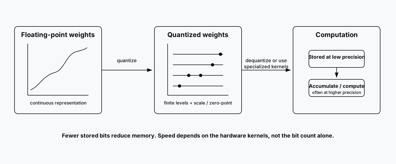
The central systems principle is

because storage, memory bandwidth, dequantization and compute kernels are distinct constraints.

Quantization maps continuous values to discrete codes

Consider a real-valued scalar $x\in\mathbb R$. A common affine quantizer maps it to an integer code

where $s>0$ is a scale and $z$ is a zero-point. Approximate dequantization is

The quantization error is

The problem is therefore not merely to compress a number. It is to choose a discrete representation so that the induced error is acceptable for the downstream computation.

Symmetric and asymmetric schemes make different assumptions

In symmetric quantization, $z=0$ or a fixed midpoint, and the representable range is centered around zero. For signed $b$-bit integers, a common scale is approximately

Asymmetric quantization permits a nonzero zero-point and can use the available range more efficiently for skewed tensors.

If $x_{\min}$ and $x_{\max}$ define the calibration range, then approximately

The extra flexibility can reduce representation error, but it can complicate hardware kernels.

One scale for an entire matrix is often too crude

For a weight matrix $W\in\mathbb R^{d\times k}$, per-tensor quantization uses one scale for the entire matrix. A single large outlier can then expand the dynamic range and waste quantization levels on the majority of smaller weights.

Per-channel quantization uses separate scales for rows or columns. Group-wise quantization partitions weights into groups of size $g$ and assigns each group its own scale.

The trade-off is

Smaller groups often preserve quality better, but they require more scale metadata and may interact differently with kernels.

Weight-only and activation quantization are different problems

A weight-only quantized layer conceptually computes

while activations remain in floating point.

This primarily reduces model storage and memory bandwidth.

If activations are also quantized,

the runtime can potentially use integer or other low-precision matrix kernels more aggressively.

Activation quantization is harder because activations are input-dependent and often contain strong outliers.

The statement "the model is 4-bit" should therefore specify which tensors are actually 4-bit.

Post-training quantization and QLoRA are different regimes

Post-training quantization starts from a trained model and finds a lower-precision representation without retraining the original model objective.

GPTQ and AWQ belong broadly to this family.

QLoRA solves a different problem. It holds the pretrained base model in a 4-bit representation while training higher-precision LoRA adapters. The low-bit representation reduces training memory; the adaptation objective remains fine-tuning.

These should not be collapsed into one category merely because all may involve four-bit weights.

Calibration data are part of the model-building process

Some quantizers use representative inputs to estimate activation statistics or reconstruction error.

Let $P_{\mathrm{cal}}$ denote the calibration distribution and $P_{\mathrm{deploy}}$ the actual deployment distribution.

If

the quantizer can optimize scales and clipping for the wrong regime.

Calibration data should therefore resemble deployment with respect to language, domain, prompt length, chat format, code versus prose, and sequence-length distribution.

Calibration is a sampling problem.

Outliers are disproportionately expensive in low precision

Suppose nearly all weights lie in $[-0.1,0.1]$, but one value is $2.0$.

A global scale wide enough to represent $2.0$ assigns relatively few discrete levels to the dense central mass.

Clipping the outlier improves resolution for most weights but creates a large error on the clipped value.

Much of modern LLM quantization is about deciding where such errors matter and protecting the important cases.

GPTQ uses approximate second-order structure

GPTQ is a post-training weight quantization method that quantizes weights while compensating for induced error using approximate curvature information.

For a linear layer

a local reconstruction objective is approximately

The quadratic structure depends on activation covariance through terms related to

GPTQ therefore does more than independently round each weight. Calibration activations influence the result.

AWQ uses activation statistics to protect salient weights

AWQ, Activation-aware Weight Quantization, uses activation information to identify weights or channels whose quantization error matters disproportionately for real inputs.

The target remains approximately

but the scaling strategy protects salient parts of the weight matrix.

The method is still commonly deployed as weight-only quantization. "Activation-aware" refers to the calibration signal used to decide which weight errors matter.

GPTQ and AWQ should be compared under controlled conditions

A useful comparison holds fixed:

• base model revision,
• nominal bit width,
• group size,
• calibration corpus,
• runtime backend,
• evaluation prompts,
• hardware.

Otherwise an apparent algorithmic difference can be caused by the surrounding configuration.

NF4 is not a generic integer quantizer

QLoRA introduced NormalFloat 4-bit, or NF4, as a nonuniform codebook designed for approximately normally distributed pretrained weights.

This makes NF4 particularly useful for storing a frozen base model during QLoRA.

A common Transformers configuration is:

1
2
3
4
5
6
7
8
9
import torch
from transformers import BitsAndBytesConfig

quantization_config = BitsAndBytesConfig(
    load_in_4bit=True,
    bnb_4bit_quant_type="nf4",
    bnb_4bit_use_double_quant=True,
    bnb_4bit_compute_dtype=torch.bfloat16,
)

The stored weights are low precision, while arithmetic can use a higher compute dtype.

Storage precision and compute precision are separate design choices.

Double quantization compresses quantization metadata

Group-wise quantization requires scale constants. Across a very large model, those constants consume nontrivial memory.

Double quantization compresses the scale values themselves.

The saving per group is small, but across billions of parameters it becomes material.

GGUF is a file format, not one quantization algorithm

GGUF is widely used in the llama.cpp ecosystem to package model tensors and metadata for portable inference.

A GGUF file can contain tensors quantized using several different schemes.

Therefore saying "the model is GGUF" does not specify the quantizer.

A complete description includes the concrete tensor quantization type and runtime.

Nominal bit-width does not equal exact bits per parameter

Real formats may include block metadata, scales, zero-points, mixed-precision tensors and higher-precision exceptions.

The realized average bits per parameter can therefore differ from the headline number.

File size and measured RAM or VRAM use are better empirical quantities than guessing from the format name.

A 4-bit model is not necessarily one quarter the file size

For $P$ parameters, pure FP16 storage is approximately

bytes.

Ideal four-bit storage would be approximately

bytes, a fourfold reduction.

Real artifacts also store quantization metadata, tokenizer files, headers and sometimes selected higher-precision tensors.

Measure the actual artifact rather than assuming the ideal ratio.

A smaller model is not automatically four times faster

Inference time can be written schematically as

Quantization primarily reduces memory traffic when inference is bandwidth-bound.

If low-bit kernels are poor or unavailable, dequantization and conversion can erase much of the expected speedup.

If the workload is compute-bound, memory compression may help little.

Hardware kernels determine whether fewer stored bits translate into throughput.

Prefill and decode can respond differently to quantization

Prompt prefill processes many tokens in parallel.

Autoregressive decoding processes one or a few new tokens while repeatedly reading model weights and KV cache.

Weight bandwidth is often more important during decoding, so quantization may produce larger gains there than during prefill.

Benchmarks should therefore report at least:

• time to first token,
• prefill throughput,
• decode throughput.

A single tokens-per-second number can hide which regime improved.

The KV cache can dominate memory at long context

Weight quantization does not automatically quantize the key-value cache.

For $L$ layers and context length $T$, KV-cache memory grows approximately linearly:

where $b$ captures the cache representation size.

At long context or large batch size, the KV cache can dominate memory even when model weights are heavily quantized.

Weight compression does not make context memory disappear.

Training still carries activation memory

QLoRA reduces the memory required to store the frozen base and dramatically reduces optimizer state relative to full fine-tuning.

It does not remove activations.

Training memory remains approximately

Gradient checkpointing targets the activation term by trading memory for extra compute.

Quantization is only one part of the training-memory budget.

Quantization error propagates through the network

Layer-local reconstruction error is useful, but a transformer is a composition of many nonlinear layers.

A perturbation introduced early in the network changes the input to later layers.

Quantization errors can therefore amplify, cancel or interact.

This is why end-to-end evaluation remains necessary even when local reconstruction metrics look excellent.

Perplexity is a useful first diagnostic

For held-out tokens $w_1,\ldots,w_T$, define

and

Compare

A small increase is encouraging.

It does not guarantee stable downstream behaviour.

Behavioural regressions can be highly nonuniform

Quantization may preserve average benchmark performance while hurting one class of tasks disproportionately.

Useful slices include:

• arithmetic,
• code generation,
• rare vocabulary,
• multilingual prompts,
• long-context retrieval,
• tool calling,
• structured output.

For task family $j$, track

Aggregate means can hide a catastrophic slice.

Calibration and evaluation sets should be separate

If AWQ or GPTQ calibration prompts also appear in the final evaluation set, the evaluation is contaminated.

Calibration affects the quantizer.

Treat it as part of model construction.

Maintain separate calibration, validation and final test sets.

Compare methods at equal resources, not merely equal bit-width

Two methods with nominal four-bit weights may have different file sizes, memory use, latency and quality.

A more useful optimization problem is

Or

Bit-width itself is not the deployment objective.

Calibration sample size should be tested

A larger calibration set estimates activation statistics more reliably, but the marginal gain eventually declines.

A simple experiment can compare

calibration sequences and track perplexity plus downstream metrics.

If performance stabilizes early, larger calibration sets may be unnecessary.

Mixed precision can protect sensitive tensors

There is no requirement that every tensor use the same bit-width.

Let tensor family $j$ use $b_j$ bits. Approximate memory becomes

The design problem is then to allocate precision where it buys the most quality.

Uniform four-bit quantization is only one point in this larger resource-allocation problem.

Embeddings and output heads may be treated differently

Some runtimes keep embedding matrices or output heads at higher precision.

That changes memory and quality.

When comparing quantized artifacts, inspect which tensors were excluded from low-bit representation.

"Four-bit model" may mean "most large linear layers are four-bit."

Quality is not universally ordered by nominal bit-width

Within one fixed quantizer, lower bit-width often reduces quality.

Across quantizers, the ordering can be different.

A well-calibrated four-bit method can outperform a poorly calibrated five-bit representation on some tasks.

Algorithm, grouping, calibration and kernels matter.

Bit-width is not a universal quality ranking.

Quantization interacts with fine-tuning order

Several workflows are possible:

1. fine-tune in high precision, then quantize;
2. quantize the base and train LoRA adapters with QLoRA;
3. merge the adapter, then quantize the merged model;
4. keep a quantized base and a separate higher-precision adapter.

They are not algebraically equivalent.

If

then generally

The artifact that will actually be served must be evaluated directly.

Hardware-specific benchmarking is mandatory

For every target platform, measure:

• peak RAM or VRAM,
• model load time,
• time to first token,
• prefill tokens per second,
• decode tokens per second,
• batch throughput,
• energy or cost when relevant.

CPU, Apple Silicon, NVIDIA GPU and cloud accelerators can rank formats differently.

The best quantizer is partly a hardware question.

A practical bitsandbytes load is simple

For Transformers, a QLoRA-style 4-bit load can look like:

1
2
3
4
5
6
7
8
9
10
11
12
13
14
15
16
17
import torch
from transformers import AutoModelForCausalLM, BitsAndBytesConfig

model_id = "your-model-id"

quantization_config = BitsAndBytesConfig(
    load_in_4bit=True,
    bnb_4bit_quant_type="nf4",
    bnb_4bit_use_double_quant=True,
    bnb_4bit_compute_dtype=torch.bfloat16,
)

model = AutoModelForCausalLM.from_pretrained(
    model_id,
    quantization_config=quantization_config,
    device_map="auto",
)

This is not an integer-only model. Low-precision storage and higher-precision computation coexist.

GPTQ and AWQ artifacts need full provenance

For an exported GPTQ or AWQ model, record at least:

• quantizer and implementation,
• bit-width,
• group size,
• calibration dataset,
• base-model revision,
• backend version,
• kernel implementation.

A filename is not enough to reproduce the experiment.

GGUF belongs in deployment benchmarking

When targeting llama.cpp, compare concrete GGUF quantization variants on the actual machine.

For variants $Q_1,Q_2,Q_3$, measure

The useful choices lie on the observed Pareto frontier.

Quantization should have acceptance criteria

Before quantizing, define acceptable degradation.

For example,

and

Otherwise the project can drift toward selecting the smallest artifact regardless of behaviour.

The right question is not how low the bit-width can go

The aggressive objective

is rarely the real system objective.

A more useful formulation is

where $U$ is task utility, $M$ memory, $T$ latency and $E$ energy or cost.

Quantization moves the model along that frontier.

The lowest bit-width is not automatically the best operating point.

References

Dettmers, T., Pagnoni, A., Holtzman, A., & Zettlemoyer, L. (2023). QLoRA: Efficient Finetuning of Quantized LLMs. Advances in Neural Information Processing Systems, 36.

Frantar, E., Ashkboos, S., Hoefler, T., & Alistarh, D. (2023). GPTQ: Accurate Post-Training Quantization for Generative Pre-trained Transformers. International Conference on Learning Representations.

Lin, J., Tang, J., Tang, H., Yang, S., Dang, X., & Han, S. (2024). AWQ: Activation-aware Weight Quantization for LLM Compression and Acceleration. Proceedings of MLSys 2024.

Hugging Face. Transformers documentation: Quantization. Accessed 21 September 2026.

Hugging Face. Transformers documentation: bitsandbytes. Accessed 21 September 2026.

ggerganov et al. llama.cpp and GGUF documentation. Accessed 21 September 2026.