Censored Labels in Supervised Learning: When ‘No Event Yet’ Is Not a Negative

A churn model starts with a database extract. Each customer has features and a status field, and the label is whether the status says churned. Customers who signed up last month have not churned, because almost nobody churns in their first month. The model learns this, reports an AUC of 0.90, and predicts a churn probability below one percent for every new signup. The retention team, which asked which new customers to call, receives a list of long-tenured accounts instead, and the model is technically doing exactly what it was trained to do.

Where the Zeros Come From

An event that has not happened by the extract date has two explanations. Either it will not happen within the horizon the business cares about, or the customer has not been observed for long enough to tell. A snapshot label writes a zero in both cases. In survival analysis this is right censoring, and it is treated as a first-class property of the data. In a classification pipeline it is invisible, because the label column contains only zeros and ones.

The censoring is not random. It is tied to signup date, so it is tied to every feature that moves with signup date: tenure, months since last activity, number of orders, plan version, acquisition channel. The label is contaminated in a way that correlates with the inputs, which is the definition of a leak.

A Simulation

Twenty thousand customers sign up at a uniform rate over three years. Each has two features that shift their true churn hazard, and the time until they churn follows a Weibull distribution whose scale depends on those features. The extract is taken at month 36. The business question is the probability of churning within twelve months of signup.

import numpy as np
from sklearn.ensemble import HistGradientBoostingClassifier
from sklearn.linear_model import LogisticRegression
from sklearn.metrics import roc_auc_score

rng = np.random.default_rng(0)
N = 20000
signup = rng.uniform(0, 36, N)             # month of signup; data extracted at month 36
x1, x2 = rng.normal(size=N), rng.normal(size=N)
lam = 18 * np.exp(-(0.8 * x1 - 0.6 * x2))  # Weibull scale in months, feature dependent
k = 1.3
T = lam * rng.weibull(k, N)                 # true months until churn
followup = 36 - signup                      # months observed
H = 12
churned_by_extract = T <= followup
p12_true = 1 - np.exp(-(H / lam) ** k)      # true 12-month churn probability
event12 = T <= H

test = rng.uniform(size=N) < 0.25
tr = ~test

# naive: label = churned by extract date; tenure at extract is a feature
Xn = np.column_stack([x1, x2, followup])
naive = HistGradientBoostingClassifier(max_iter=200, learning_rate=0.05,
                                       random_state=0).fit(Xn[tr], churned_by_extract[tr])
p_naive = naive.predict_proba(Xn[test])[:, 1]

The naive model is the one most teams build. Its label is the status field, and tenure is included because it is available and predictive.

# fixed horizon: only customers observed for 12 months; label = churned within 12
full = followup >= H
Xf = np.column_stack([x1, x2])
fixed = HistGradientBoostingClassifier(max_iter=200, learning_rate=0.05,
                                       random_state=0).fit(Xf[tr & full], event12[tr & full])
p_fixed = fixed.predict_proba(Xf[test])[:, 1]

# discrete-time hazard: one row per customer-month up to min(churn, follow-up, 12)
def person_months(idx):
    rows, ys = [], []
    for i in idx:
        last = int(np.ceil(min(T[i], followup[i], H)))
        for m in range(1, max(last, 1) + 1):
            rows.append((x1[i], x2[i], m))
            ys.append(int(T[i] <= m and T[i] > m - 1 and m <= followup[i] + 1e-9))
    return np.array(rows), np.array(ys)

def design(rows):
    m = rows[:, 2].astype(int)
    return np.column_stack([rows[:, :2], np.eye(H)[m - 1]])   # features + month dummies

R, Y = person_months(np.where(tr)[0])
haz = LogisticRegression(C=10.0, max_iter=2000).fit(design(R), Y)
print(f"person-month rows used by the hazard model: {len(R):,} from {tr.sum():,} customers "
      f"(incl. {np.sum(tr & ~full):,} with under 12 months)")

def p12_hazard(idx):
    surv = np.ones(len(idx))
    for m in range(1, H + 1):
        rows = np.column_stack([x1[idx], x2[idx], np.full(len(idx), m)])
        surv *= 1 - haz.predict_proba(design(rows))[:, 1]
    return 1 - surv
p_haz = p12_hazard(np.where(test)[0])

The fixed-horizon model changes the label to what the business asked for and drops every customer who cannot yet have that label. The hazard model changes the unit of analysis instead: one row per customer per month, a binary outcome of churning in that month, and a month effect, so that a customer with four months of follow-up contributes four rows and then stops without being called a negative. The twelve-month probability is one minus the product of twelve monthly survival probabilities.

ten = followup[test]
bins = [(0, 3), (3, 6), (6, 12), (12, 24), (24, 36)]
print("\ncohort     n     true    naive   fixed   hazard")
for lo, hi in bins:
    s = (ten >= lo) & (ten < hi)
    print(f"{lo:>2}-{hi:<5} {s.sum():>5}   {p12_true[test][s].mean():.3f}   "
          f"{p_naive[s].mean():.3f}   {p_fixed[s].mean():.3f}   {p_haz[s].mean():.3f}")

Months since signup	Customers	True 12-month churn	Naive	Fixed horizon	Hazard
0 to 3	410	0.501	0.089	0.505	0.495
3 to 6	415	0.456	0.219	0.465	0.450
6 to 12	890	0.476	0.396	0.478	0.469
12 to 24	1,700	0.484	0.607	0.488	0.477
24 to 36	1,633	0.490	0.737	0.494	0.483

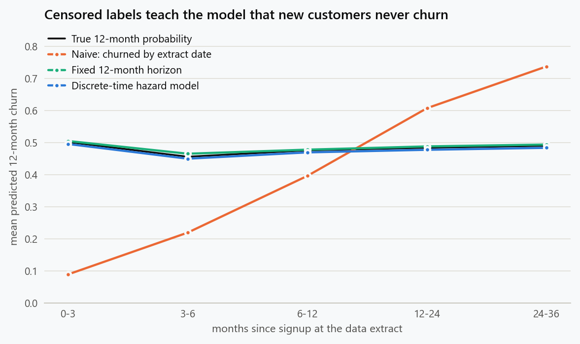
The true twelve-month churn probability is about 48 percent in every cohort, because signup date has nothing to do with risk in this simulation. The naive model says 9 percent for the newest customers and 74 percent for the oldest. It has learned the probability of having churned by the extract, which for a customer observed for two months is the two-month churn probability and for a customer observed for thirty months is the thirty-month one, and it reports that as if it were the twelve-month risk. The other two models are flat at the truth.

print("\nagainst the true 12-month outcome, all test customers:")
for name, p in (("naive", p_naive), ("fixed", p_fixed), ("hazard", p_haz)):
    print(f"  {name:<7} AUC {roc_auc_score(event12[test], p):.3f}   "
          f"mean |pred - true prob| {np.mean(np.abs(p - p12_true[test])):.3f}")
print("naive model's AUC on its own labels:",
      round(roc_auc_score(churned_by_extract[test], p_naive), 3))
print("brand-new customer with average features: naive",
      round(naive.predict_proba([[0.0, 0.0, 0.0]])[0, 1], 3),
      "| true 12-month probability", round(1 - np.exp(-(H / 18) ** k), 3))

Model	AUC against the true 12-month outcome	Mean absolute error in probability
Naive	0.764	0.193
Fixed horizon	0.839	0.051
Hazard	0.849	0.007

The naive model’s AUC against its own labels is 0.896. Against the outcome the business asked about it is 0.764, and its probabilities are off by 19 points on average. For a brand-new customer with average features it predicts a churn probability of 0.006 against a true value of 0.446, a factor of about seventy. None of this is visible from inside the pipeline: the training labels, the validation labels and the test labels all have the same censoring, so every metric the pipeline computes agrees that the model is excellent.

The gap between the fixed-horizon and hazard models in the last table is partly model class rather than label construction. The hazard model here is a logistic regression whose form matches the simulation closely, while the fixed-horizon model is a gradient boosting classifier with more variance. The comparison that matters is between the naive model and either of the others.

The Feature That Leaks Time

Tenure at extract did the damage in the naive model, and removing it does not undo it. Without tenure, the model can no longer express the bias per cohort, so it averages it: the snapshot label’s positive rate is 42 percent against a true twelve-month rate of 49 percent, and the model predicts around the lower figure for everyone. The label is still the wrong label. Tenure merely made the wrongness visible by cohort, and any other feature that moves with signup date, such as plan version, acquisition channel or number of orders, carries the same information more quietly.

There is a second, subtler version. Features measured at the extract, such as days since last login, are computed on a different clock for each customer. For a customer who churned a year ago, days since last login is enormous, and it is enormous because they churned, not before it. A feature computed after the event it is supposed to predict is a leak of the ordinary kind, and snapshot pipelines produce it by default. Features have to be computed as of the reference time the label is defined from, not as of the extract.

Three Fixes

Approach	Data used	Tooling	Output	Cost
Fixed horizon	Customers observed at least $H$	Any classifier	Probability of the event within $H$	Discards recent cohorts; lags behind change
Discrete-time hazard	Every customer, every observed period	Any classifier on person-period rows	Full curve; any horizon	Rows multiply; needs month effects
Censoring weights	Every customer with a determinable label	Any classifier, with sample weights	Probability within $H$	Needs a censoring model; noisy weights near the horizon

Fixed horizon is the smallest change. Define the label as the event within $H$ of a reference time, require follow-up of at least $H$, compute features as of the reference time, and train a classifier. It answers the business question exactly and needs no new tooling. Its cost is data: in the simulation, 5,014 of 14,952 training customers had less than twelve months of follow-up and were dropped, and they were the most recent ones, which are the ones most representative of current conditions.

Discrete-time hazard keeps them. The 14,952 customers produced 115,084 customer-month rows, and a customer with four months of history contributed four rows to the estimation of the early hazards without being asked about the eighth month. The model is an ordinary classifier on ordinary rows, which means gradient boosting or a neural network can replace the logistic regression without changing the construction, and it produces the whole survival curve, so the twelve-month question and the three-month question come from one fit. Singer and Willett’s account of this construction is the standard reference.

Censoring weights take a middle path. Each customer whose twelve-month label can be determined is kept, and weighted by the inverse of the probability of being observed that long, estimated from the censoring distribution. Customers observed for a long time stand in for the similar customers who were censored early. It keeps the classifier and the label unchanged and uses more of the data than the fixed horizon does, at the cost of a censoring model and of large weights where few customers were observed long enough.

The Evaluation Is Censored Too

Fixing the training labels is not enough, because the test set was drawn from the same snapshot.

print("\n12-month churn rate among test customers")
print(f"  true                              {event12[test].mean():.3f}")
print(f"  observed, all customers           {(churned_by_extract & (T <= H))[test].mean():.3f}")
print(f"  observed, >= 12 months follow-up  {event12[test & full].mean():.3f}")

The true twelve-month churn rate in the test set is 48.6 percent. Counted from the snapshot across all test customers it is 41.8 percent, because recent customers who will churn within twelve months have not done so yet. Restricted to customers with at least twelve months of follow-up it is 49.0 percent. A model with correct probabilities evaluated against the snapshot labels looks overconfident, and a model calibrated to the snapshot labels looks right. The evaluation has to be restricted to fully observed customers, or use the censoring-weighted versions of the usual metrics: the inverse-probability-weighted Brier score of Graf and colleagues and the time-dependent AUC of Uno and colleagues exist for exactly this.

Restricting the evaluation to customers observed for the full horizon means the evaluation is always at least $H$ behind the present. That is a real cost, and it is the honest one. A model whose evaluation claims to know how it does on this month’s signups is claiming to know this month’s future.

Same Problem, Other Names

The snapshot label appears wherever an event has a time and the data has an extract date.

• Predictive maintenance. Machines that have not failed yet are labeled healthy, and the newest machines are the healthiest of all.
• Credit risk. Loans that have not defaulted include loans that are two months old. Vintage analysis, which compares loans at the same age, is the credit industry’s fixed-horizon construction.
• Readmission within 30 days, computed on an extract that includes patients discharged last week.
• Lead conversion, where leads created yesterday are counted as not converted.
• Employee attrition, where the last cohort of hires has a perfect retention record.

The general rule is the same in each. The label is the event within a horizon of a reference time, it is defined only for records observed for at least that horizon past the reference time, and the features are computed as of the reference time. Anything else is a model of the extract date.

What to Do

1. Write the label as a sentence with a horizon and a reference time before writing any code: “churn within twelve months of signup”, not “status equals churned”.
2. Check the positive rate by observation time. If it rises with tenure at extract, the label is censored.
3. Pick a construction: fixed horizon for simplicity, discrete-time hazard to use all the data and get the whole curve, censoring weights to keep an existing classifier.
4. Compute features as of the reference time, never as of the extract.
5. Evaluate on records with full follow-up, or with censoring-weighted metrics, and accept that the evaluation lags the present by the horizon.
6. Treat the model’s own metrics with suspicion when training, validation and test share a snapshot. An AUC of 0.90 on a censored label is a measurement of how well the model has learned the extract date.

References

• Kalbfleisch, J. D., & Prentice, R. L. (2002). The Statistical Analysis of Failure Time Data (2nd ed.). Wiley.
• Singer, J. D., & Willett, J. B. (1993). It’s about time: using discrete-time survival analysis to study duration and the timing of events. Journal of Educational Statistics, 18(2), 155-195.
• Graf, E., Schmoor, C., Sauerbrei, W., & Schumacher, M. (1999). Assessment and comparison of prognostic classification schemes for survival data. Statistics in Medicine, 18(17-18), 2529-2545.
• Uno, H., Cai, T., Tian, L., & Wei, L. J. (2007). Evaluating prediction rules for t-year survivors with censored regression models. Journal of the American Statistical Association, 102(478), 527-537.
• Kvamme, H., Borgan, Ø., & Scheel, I. (2019). Time-to-event prediction with neural networks and Cox regression. Journal of Machine Learning Research, 20(129), 1-30.
• Wang, P., Li, Y., & Reddy, C. K. (2019). Machine learning for survival analysis: a survey. ACM Computing Surveys, 51(6), 1-36.