Topics
One plant got the new maintenance regime. One region got the price change. One store got the new layout. In each case the intervention happened once, on one unit, and nothing was randomised. The question is what would have happened to that unit without it, and there are two common answers, both wrong. Before-after compares the unit with its own past, and fails whenever anything else changed over the same period. Difference-in-differences compares the unit's change with everyone else's, and fails whenever the unit was not on everyone else's trajectory to begin with, which is usually why it was chosen for the intervention.
Synthetic control takes the second idea and repairs its weakness. Instead of comparing against the average of the untreated units, it compares against a weighted average of them, with the weights chosen so that the combination tracked the treated unit before the intervention. If a combination of other plants behaved like this plant for three years, it is a fair guess at how this plant would have behaved in the fourth.
The Idea
Let unit 1 be treated from period $T_0 + 1$, and units $2, \dots, J+1$ be untreated donors. Synthetic control finds weights $w_2, \dots, w_{J+1}$, non-negative and summing to one, that minimise the distance between the treated unit's pre-intervention outcomes and the weighted combination of the donors'. The estimated effect at each post-intervention period is
The constraints matter. Because the weights are non-negative and sum to one, the synthetic unit is an interpolation of real donors, never an extrapolation beyond them, and the weights are readable: the synthetic plant is 38 percent plant B, 30 percent plant F and so on. Abadie, Diamond and Hainmueller showed that when outcomes follow a factor model, common time-varying factors with unit-specific loadings, a combination that matches the treated unit over a long enough pre-period also matches its unobserved loadings, and therefore its counterfactual path.
A Simulation With a Known Effect
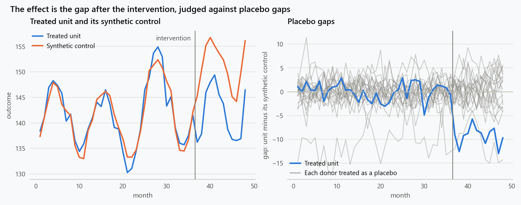
Twenty donor units and one treated unit are driven by two common factors, a drifting trend and a seasonal cycle, each unit with its own loadings and its own level. The treated unit follows the trend more strongly than the average donor: it is a growing plant. From month 37 its outcome drops by eight units.
1
2
3
4
5
6
7
8
9
10
11
12
13
14
15
16
17
18
19
20
21
22
23
24
25
26
27
28
29
30
31
32
33
34
35
import numpy as np
from scipy.optimize import minimize

def simulate(seed, n_donors=20, pre=36, post=12, effect=-8.0, treated_loads=(1.2, 0.9)):
    r = np.random.default_rng(seed)
    T = pre + post
    trend = np.cumsum(r.normal(0.3, 1.0, T)) + 100            # a common trending factor
    season = 10 * np.sin(np.arange(T) * 2 * np.pi / 12)        # a common seasonal factor
    f = np.column_stack([trend, season])
    loads = r.uniform(0.3, 1.5, (n_donors + 1, 2))             # donors: how strongly each follows the factors
    loads[0] = treated_loads                                   # the treated unit: grows faster than the average donor
    mu = r.uniform(-20, 20, n_donors + 1)
    Y = mu[:, None] + loads @ f.T + r.normal(0, 2.0, (n_donors + 1, T))
    Y[0, pre:] += effect                                       # treatment on unit 0 from month `pre`
    return Y, pre

def synth_weights(y_treated, Y_donors):
    k = Y_donors.shape[0]
    obj = lambda w: np.mean((y_treated - w @ Y_donors) ** 2)
    res = minimize(obj, np.full(k, 1 / k), method="SLSQP", bounds=[(0, 1)] * k,
                   constraints={"type": "eq", "fun": lambda w: w.sum() - 1}, options={"maxiter": 500})
    return res.x

def estimate(Y, pre):
    w = synth_weights(Y[0, :pre], Y[1:, :pre])
    synth = w @ Y[1:]
    return w, synth, Y[0] - synth

Y, pre = simulate(0)
w, synth, gap = estimate(Y, pre)
print(f"donors with weight > 0.01: {np.sum(w > 0.01)}; largest weights {np.sort(w)[::-1][:4].round(2)}")
print(f"pre-period RMSPE {np.sqrt(np.mean(gap[:pre]**2)):.2f}; post-period mean gap {gap[pre:].mean():.2f} (true effect -8.0)")
naive = Y[0, pre:].mean() - Y[0, :pre].mean()
did = naive - (Y[1:, pre:].mean() - Y[1:, :pre].mean())
print(f"naive before-after {naive:+.2f}; difference-in-differences vs donor average {did:+.2f}")
| Estimator | Estimated effect | Truth |
|---|---|---|
| Before-after on the treated unit | +0.30 | -8.0 |
| Difference-in-differences against the donor average | -6.64 | -8.0 |
| Synthetic control | -9.29 | -8.0 |
Before-after finds nothing, because the rising trend over the post-period cancels the drop. Difference-in-differences finds two thirds of the effect, because the treated unit was growing faster than the donor average, so the donors understate what it would have done on its own. Synthetic control puts positive weight on four donors, with the largest at 0.38, matches the pre-period to a root mean squared error of 1.81 against noise with standard deviation 2, and estimates -9.29.
Inference Without a Standard Error
With one treated unit there is no sampling distribution to appeal to, and the method's inference is a permutation argument. Apply the same procedure to each donor as if it had been the treated one, and see whether the real treated unit's post-intervention gap stands out from the placebo gaps. The statistic is the ratio of post-period to pre-period root mean squared prediction error, which penalises units whose large post-period gap merely continues a poor pre-period fit.
1
2
3
4
5
6
7
8
9
10
11
12
13
14
15
ratios = []
for j in range(Y.shape[0]):
    others = np.delete(Y, j, axis=0)
    wj = synth_weights(Y[j, :pre], others[:, :pre])
    g = Y[j] - wj @ others
    ratios.append(np.sqrt(np.mean(g[pre:]**2)) / np.sqrt(np.mean(g[:pre]**2)))
ratios = np.array(ratios)
rank = 1 + np.sum(ratios[1:] >= ratios[0])
print(f"placebo in space: treated post/pre RMSPE ratio {ratios[0]:.1f}; donors' median {np.median(ratios[1:]):.1f}, "
      f"max {ratios[1:].max():.1f}; rank {rank} of {len(ratios)} -> p = {rank/len(ratios):.3f}")

fake = pre - 12
wt = synth_weights(Y[0, :fake], Y[1:, :fake])
gap_t = Y[0, :pre] - wt @ Y[1:, :pre]
print(f"placebo in time (fake treatment at month {fake}): mean gap in the fake post-period {gap_t[fake:].mean():+.2f}")
The treated unit's ratio is 5.2. The donors' ratios have a median of 1.2 and a maximum of 2.0. The treated unit ranks first of twenty-one, which gives a permutation p-value of 0.048, and that number deserves a comment: with twenty donors, one in twenty-one is the smallest p-value the test can produce. The resolution of the inference is set by the size of the donor pool, and a study with eight donors cannot reach conventional significance whatever the effect.
The placebo in time is the complementary check. Pretend the intervention happened at month 24, fit the weights on the first 24 months, and look at the gap over months 25 to 36, when nothing happened. It is +0.72, against an estimated effect of -9.29. A method that finds large effects where there are none is not to be trusted where there might be.
Bias and Precision Over Two Hundred Replications
One dataset shows one outcome. Repeating the simulation with fresh noise, factors and donors shows what each estimator does on average, and how the length of the pre-period matters.
| Pre-intervention months | Synthetic control | Difference-in-differences | Before-after | Median pre-period fit |
|---|---|---|---|---|
| 6 | -7.80 (sd 1.76) | -7.23 (sd 1.48) | -10.26 (sd 3.05) | 0.99 |
| 12 | -7.63 (sd 1.65) | -6.92 (sd 1.14) | -3.69 (sd 3.27) | 1.39 |
| 36 | -7.79 (sd 1.34) | -5.88 (sd 1.57) | +0.72 (sd 4.89) | 1.91 |
The true effect is -8. Synthetic control is close to unbiased at every pre-period length and its spread shrinks as the pre-period grows. Difference-in-differences is biased, and the bias grows with the length of the window, from under one unit at six months to over two at thirty-six, because the treated unit's faster trend has longer to accumulate against the donor average. Before-after is not an estimator of anything: its answer depends entirely on what the trend did over the window.
The bias pattern of difference-in-differences explains a familiar experience. A short before-after window sometimes gives a reasonable answer, and a long one gives nonsense, and the reason is not that short windows are better but that a trend has less room to act in them. Synthetic control removes the trend by matching it, and the length of the window then only helps.
When It Fails
The method has one central requirement, and one diagnostic for it. The treated unit has to be reproducible as a convex combination of donors: inside their hull, in the space of whatever drives the outcome. When it is not, the weights cannot match the pre-period, and the estimate is meaningless.
1
2
3
4
5
6
7
8
sc_, fits = [], []
for s in range(200):
    Yr, p = simulate(3000 + s, treated_loads=(2.2, 2.0))       # loads beyond every donor
    _, _, g = estimate(Yr, p)
    sc_.append(g[p:].mean())
    fits.append(np.sqrt(np.mean(g[:p]**2)))
print(f"treated unit outside the donor hull: SC mean {np.mean(sc_):.2f}, sd {np.std(sc_):.2f}; "
      f"median pre-RMSPE {np.median(fits):.1f}")
With the treated unit's loadings set beyond every donor's, the estimated effect averages +71.6 against a truth of -8, and the pre-period fit has a root mean squared error of 72.6 against a noise level of 2. The diagnostic is unmissable, provided anyone looks at it. The rule is that a post-period gap is not to be reported without the pre-period fit beside it, and that a pre-period fit much larger than the noise in the outcome means there is no valid counterfactual, whatever the post-period shows. Abadie's own guidance is that the method should not be used in that case. The augmented synthetic control of Ben-Michael, Feller and Rothstein corrects for moderate pre-period imbalance with an outcome model, and is the tool for the intermediate case where the fit is imperfect but not hopeless.
Three other failure modes are common in operational data.
Spillovers. If the intervention on one plant changed the load at neighbouring plants, those plants are not untreated, and including them as donors contaminates the counterfactual. Donors that could plausibly have been affected should be excluded before fitting.
Anticipation. If the unit began to change before the official start date, because staff knew the change was coming, fitting the weights on a pre-period that includes the anticipation matches the wrong path. The intervention date should be moved back to the point at which behaviour could have changed.
Many donors, few pre-periods. With twenty donors and six pre-periods, weights can be found that match noise. In this simulation the noise was small and the six-month estimates held up, but with noisier outcomes the fit is spurious and the placebo test is what exposes it: the donors then also achieve good fits and large post-period gaps, and the treated unit no longer stands out.
Where It Applies
The method was built for regions and countries, but its natural home in industry is anything that happens once to one of several similar units: a maintenance regime at one plant among a fleet, a pricing change in one region, a layout in one store, a configuration change on one server cluster, a marketing campaign in one city. The requirement is a set of comparable untreated units with a shared history long enough to match on, which most fleets and networks have.
What it cannot deliver is external validity. The estimate is the effect on this unit, and generalising it to the fleet is a separate argument.
What to Do
- Assemble the donor pool from units that were not affected, directly or through spillover, and that are plausibly similar to the treated unit.
- Fit the weights on the pre-period and report the pre-period fit and the weights. A fit far worse than the outcome's noise ends the analysis.
- Run the placebo in space and report the treated unit's rank among the donors, remembering that the donor count sets the finest p-value available.
- Run the placebo in time at a date before the intervention and expect nothing.
- Leave out the heaviest donor and refit; an estimate that hinges on one donor is fragile.
- Report the effect as a path, period by period, rather than as one number, since the shape of the gap is part of the evidence.
- Use the augmented estimator when the pre-period fit is imperfect, and say so.
The method does not manufacture a control group. It makes explicit, and testable, the assumption that every before-after comparison makes silently: that the unit would have followed some path, and that we know what it was.
The figure generator in the blog-reproducibility repository reproduces this article's figure; run it with --dry-run to print the numbers behind the figure without writing an image.
References
- Abadie, A., & Gardeazabal, J. (2003). The economic costs of conflict: a case study of the Basque Country. American Economic Review, 93(1), 113-132.
- Abadie, A., Diamond, A., & Hainmueller, J. (2010). Synthetic control methods for comparative case studies: estimating the effect of California's tobacco control program. Journal of the American Statistical Association, 105(490), 493-505.
- Abadie, A. (2021). Using synthetic controls: feasibility, data requirements, and methodological aspects. Journal of Economic Literature, 59(2), 391-425.
- Ben-Michael, E., Feller, A., & Rothstein, J. (2021). The augmented synthetic control method. Journal of the American Statistical Association, 116(536), 1789-1803.
- Arkhangelsky, D., Athey, S., Hirshberg, D. A., Imbens, G. W., & Wager, S. (2021). Synthetic difference-in-differences. American Economic Review, 111(12), 4088-4118.
- Doudchenko, N., & Imbens, G. W. (2016). Balancing, regression, difference-in-differences and synthetic control methods: a synthesis. arXiv:1610.07748.
Embed interactive plots, widgets, and demos using <figure>, <iframe>, or <div class="interactive-embed"> containers. Ensure each embed includes descriptive captions for accessibility.
How to cite
Use the quick export buttons to save citations for reference managers or copy the formatted text directly.
Diogo Ribeiro (2025). Synthetic Control: Evaluating an Intervention on One Unit. Faculty of Media Arts and Design, Technical University of Porto. https://diogoribeiro7.github.io/data-science/synthetic_control_single_unit_interventions/.