Real-world Case Studies

This vignette illustrates how to incorporate heteroTests into real analyses. Each case study follows a workflow of model specification, diagnostic testing, visualisation, and interpretation.

Case study 1: Seismic station counts

R's built-in quakes dataset records 1,000 seismic events near Fiji. We regress the number of reporting stations on event magnitude and depth, and inspect the residual dispersion. The response is a count, so its variance is expected to rise with its mean.

quakes_model <- lm(stations ~ mag + depth, data = quakes)
summary(quakes_model)
#>
#> Call:
#> lm(formula = stations ~ mag + depth, data = quakes)
#>
#> Residuals:
#>     Min      1Q  Median      3Q     Max
#> -46.506  -6.996  -0.453   6.643  47.259
#>
#> Coefficients:
#>               Estimate Std. Error t value Pr(>|t|)
#> (Intercept) -1.920e+02  4.332e+00 -44.335  < 2e-16 ***
#> mag          4.791e+01  9.016e-01  53.135  < 2e-16 ***
#> depth        1.318e-02  1.685e-03   7.822 1.32e-14 ***
#> ---
#> Signif. codes:  0 '***' 0.001 '**' 0.01 '*' 0.05 '.' 0.1 ' ' 1
#>
#> Residual standard error: 11.17 on 997 degrees of freedom
#> Multiple R-squared:  0.7404, Adjusted R-squared:  0.7399
#> F-statistic:  1422 on 2 and 997 DF,  p-value: < 2.2e-16

Formal diagnostics flag heteroscedasticity consistent with the classical literature on this dataset.

white_q <- performWhiteTest(quakes_model, quakes)
#> [INFO] Running White test
#> [INFO] White test completed: statistic = 125.558 df = 5 p = 0
bp_q <- performBPTest(quakes_model, quakes)
#> [INFO] Running Breusch-Pagan test
koenker_q <- performKoenkerTest(quakes_model, quakes)
#> [INFO] Running Koenker test
list(White = white_q, Breusch_Pagan = bp_q, Koenker = koenker_q)
#> $White
#>
#>  White's test for heteroscedasticity
#>
#> data:  quakes_model
#> X-squared = 125.56, df = 5, p-value < 2.2e-16
#> alternative hypothesis: heteroscedasticity present
#>
#>
#> $Breusch_Pagan
#>
#>  Breusch-Pagan test for heteroscedasticity
#>
#> data:  stations ~ mag + depth
#> X-squared = 191.93, df = 2, p-value < 2.2e-16
#>
#>
#> $Koenker
#>
#>  Koenker studentized Breusch-Pagan test
#>
#> data:  stations ~ mag + depth
#> X-squared = 111.31, df = 2, p-value < 2.2e-16

plot_data <- data.frame(
  fitted = fitted(quakes_model),
  residual = resid(quakes_model),
  mag = quakes$mag
)

ggplot(plot_data, aes(x = fitted, y = residual, colour = mag)) +
  geom_point(alpha = 0.7) +
  scale_colour_viridis_c(option = "C") +
  geom_smooth(se = FALSE, colour = "black") +
  labs(
    x = "Fitted values",
    y = "Residuals",
    colour = "mag",
    title = "Heteroscedasticity in reported station counts"
  ) +
  theme_minimal()
#> `geom_smooth()` using method = 'gam' and formula = 'y ~ s(x, bs = "cs")'

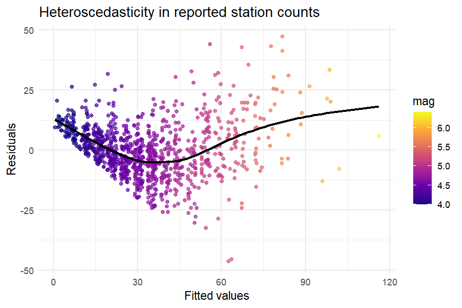
Interpretation. All three tests reject homoskedasticity. The residual plot reveals wider dispersion at higher predicted counts and for events of larger mag. Weighted least squares is a common remedy.

wls_q <- fitWLS(quakes_model)

# Compare like with like: the residual variance across thirds of the fitted
# range, unweighted for OLS and weighted for WLS.
third <- cut(fitted(quakes_model), 3, labels = c("low", "mid", "high"))
rbind(
  OLS_resid_var = round(tapply(residuals(quakes_model)^2, third, mean), 1),
  WLS_weighted_resid_var = round(
    tapply((residuals(wls_q) * sqrt(weights(wls_q)))^2, third, mean), 3))
#>                          low     mid    high
#> OLS_resid_var          80.30 196.900 526.400
#> WLS_weighted_resid_var 84.39 123.118 248.911

The unweighted variance climbs steeply across the fitted range -- a 6.6-fold spread -- which is the heteroscedasticity the tests detected. Weighting cuts that to roughly 3-fold: a real improvement, and not a complete one, because the variance model is an approximation rather than the truth.

fitWLS() estimates the weights by regressing log(e^2) on the model's design matrix and inverting the fitted variance, so the flattening above reflects the data rather than the arithmetic. That has been true only since 0.9.0; before then the weights were the raw inverse squared residuals, which put almost all the weight on a handful of well-fitted points and made standard errors from the fit unusable. For a count response like this one, a quasi-Poisson GLM models the mean-variance link directly and is worth comparing against.

Case study 2: Income volatility in simulated survey data

The hetero_data sample mimics survey responses with variance inflation driven by the regressor x.

data(hetero_data, package = "heteroTests")
survey_model <- lm(y ~ x, data = hetero_data)
summary(survey_model)
#>
#> Call:
#> lm(formula = y ~ x, data = hetero_data)
#>
#> Residuals:
#>     Min      1Q  Median      3Q     Max
#> -5.5452 -0.7444  0.0477  1.0228  5.6119
#>
#> Coefficients:
#>             Estimate Std. Error t value Pr(>|t|)
#> (Intercept)   0.7378     0.3257   2.265   0.0257 *
#> x             2.5752     0.5389   4.779 6.19e-06 ***
#> ---
#> Signif. codes:  0 '***' 0.001 '**' 0.01 '*' 0.05 '.' 0.1 ' ' 1
#>
#> Residual standard error: 1.619 on 98 degrees of freedom
#> Multiple R-squared:  0.189,  Adjusted R-squared:  0.1807
#> F-statistic: 22.84 on 1 and 98 DF,  p-value: 6.193e-06

HeteroDiagnostic() orchestrates multiple tests and visualisations.

survey_diag <- HeteroDiagnostic(survey_model, hetero_data)
runDiagnostics(survey_diag$model, survey_diag$data, tests = c("white", "breusch_pagan"))
#> [INFO] Running White test
#> [INFO] White test completed: statistic = 11.7509 df = 2 p = 0.0028
#> [INFO] Running Breusch-Pagan test
#> $white
#>
#>  White's test for heteroscedasticity
#>
#> data:  model
#> X-squared = 11.751, df = 2, p-value = 0.002808
#> alternative hypothesis: heteroscedasticity present
#>
#>
#> $breusch_pagan
#>
#>  Breusch-Pagan test for heteroscedasticity
#>
#> data:  y ~ x
#> X-squared = 22.407, df = 1, p-value = 2.206e-06
#>
#>
#> $vif
#> x
#> 1
#>
#> $reset
#>
#>  RESET test for nonlinearity
#>
#> data:  y ~ x
#> F = 0.19163, df1 = 2, df2 = 96, p-value = 0.8259
#>
#>
#> $influence
#> $influence$cooks_distance
#>            1            2            3            4            5            6
#> 1.278638e-03 2.668070e-02 1.026024e-02 5.579106e-03 6.349527e-06 2.946038e-04
#>            7            8            9           10           11           12
#> 4.094356e-03 3.482987e-04 7.177781e-02 4.287314e-04 5.548406e-04 1.200565e-04
#>           13           14           15           16           17           18
#> 7.046439e-03 8.347577e-03 2.196691e-03 4.693749e-02 1.840612e-03 5.256587e-03
#>           19           20           21           22           23           24
#> 3.506653e-03 2.425103e-03 3.708640e-02 6.722310e-05 1.062325e-02 3.964618e-02
#>           25           26           27           28           29           30
#> 1.375270e-04 1.422646e-03 2.445764e-03 3.471924e-03 3.143240e-03 2.806895e-02
#>           31           32           33           34           35           36
#> 2.360327e-02 4.454703e-04 5.432384e-05 3.228093e-04 9.956784e-04 5.019479e-03
#>           37           38           39           40           41           42
#> 1.752426e-04 2.533352e-06 1.900465e-02 3.721407e-03 7.782027e-03 8.725955e-04
#>           43           44           45           46           47           48
#> 2.814303e-03 6.358229e-02 4.810743e-03 3.504117e-02 3.936733e-02 1.637565e-02
#>           49           50           51           52           53           54
#> 6.669138e-05 2.323281e-03 5.969784e-03 4.538897e-03 3.694097e-03 4.572941e-02
#>           55           56           57           58           59           60
#> 1.570581e-04 5.468116e-06 2.041706e-03 1.750695e-05 3.239294e-04 4.294907e-05
#>           61           62           63           64           65           66
#> 7.328273e-05 9.144212e-06 4.237541e-03 1.562168e-03 6.517162e-02 1.497437e-04
#>           67           68           69           70           71           72
#> 6.196408e-04 1.265350e-01 1.886956e-02 2.507069e-04 2.977826e-03 4.955547e-03
#>           73           74           75           76           77           78
#> 2.632780e-04 4.288032e-03 9.415246e-05 2.688959e-03 2.835162e-05 1.507058e-02
#>           79           80           81           82           83           84
#> 7.080331e-03 1.031802e-03 1.533660e-03 2.658511e-04 7.930212e-06 8.215338e-03
#>           85           86           87           88           89           90
#> 2.575105e-02 6.758119e-03 7.811066e-07 6.629211e-03 6.675177e-05 2.424104e-06
#>           91           92           93           94           95           96
#> 1.876505e-04 2.782585e-04 2.957596e-04 6.822842e-04 8.685014e-03 1.205923e-02
#>           97           98           99          100
#> 6.633159e-04 9.462862e-04 4.488622e-03 7.988868e-03
#>
#> $influence$influential
#>  9 16 44 54 65 68
#>  9 16 44 54 65 68
#>
#> $influence$cutoff
#> [1] 0.04081633
performGlejserTest(survey_model, hetero_data, "x")
#> [INFO] Running Glejser test
#>
#>  Glejser test for heteroscedasticity (robust to asymmetric errors)
#>
#> data:  y ~ x
#> t = 5.0343, df = 98, p-value = 2.181e-06

plot(survey_diag, plots = c("spread_level"))
#> $spread_level
#> `geom_smooth()` using formula = 'y ~ x'

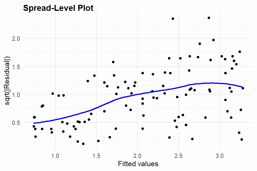
Interpretation. The Glejser test (corrected for asymmetric errors, the default) and the scale-location plot both indicate that variance increases with x. Depending on the modelling goal, analysts might log transform the response or model the variance explicitly (e.g. via lm weights or glm with a variance function).

Case study 3: Engineering reliability assessment

The diagnostic_data dataset contains correlated predictors representing engineering stress measures. Nonlinear effects and multicollinearity can mask heteroscedasticity. We run the broader diagnostic suite to capture interactions between variance and structure checks.

data(diagnostic_data, package = "heteroTests")
diagnostic_ext <- transform(diagnostic_data, x1_sq = x1^2)
engineering_model <- lm(y ~ x1 + x1_sq + x2, data = diagnostic_ext)
engineer_results <- runDiagnostics(engineering_model, diagnostic_ext,
  tests = c("breusch_pagan", "koenker")
)
#> [INFO] Running Breusch-Pagan test
#> [INFO] Running Koenker test
safe_htest <- function(fn, method) {
  tryCatch(
    fn(),
    error = function(e) {
      message(method, " unavailable: ", e$message)
      structure(
        list(
          statistic = c(statistic = NA_real_),
          parameter = NA_real_,
          p.value = NA_real_,
          method = paste0(method, " (failed)"),
          data.name = deparse(stats::formula(engineering_model))
        ),
        class = "htest"
      )
    }
  )
}
white_engineering <- safe_htest(
  function() performWhiteTest(engineering_model, diagnostic_ext, cross_products = FALSE),
  "White test"
)
#> [INFO] Running White test
#> [INFO] White test: dropped 1 collinear auxiliary term(s); using df = 5.
#> [INFO] White test completed: statistic = 6.4178 df = 5 p = 0.2677
bp_engineering <- safe_htest(
  function() performBPTest(engineering_model, diagnostic_ext),
  "Breusch-Pagan test"
)
#> [INFO] Running Breusch-Pagan test
koenker_engineering <- safe_htest(
  function() performKoenkerTest(engineering_model, diagnostic_ext),
  "Koenker test"
)
#> [INFO] Running Koenker test
harvey_engineering <- safe_htest(
  function() performHarveyTest(engineering_model),
  "Harvey test"
)
#> [INFO] Running Harvey test
engineer_tests <- list(
  white = white_engineering,
  breusch_pagan = bp_engineering,
  koenker = koenker_engineering,
  harvey = harvey_engineering
)
engineer_tests
#> $white
#>
#>  White's test for heteroscedasticity
#>
#> data:  engineering_model
#> X-squared = 6.4178, df = 5, p-value = 0.2677
#> alternative hypothesis: heteroscedasticity present
#>
#>
#> $breusch_pagan
#>
#>  Breusch-Pagan test for heteroscedasticity
#>
#> data:  y ~ x1 + x1_sq + x2
#> X-squared = 2.65, df = 3, p-value = 0.4488
#>
#>
#> $koenker
#>
#>  Koenker studentized Breusch-Pagan test
#>
#> data:  y ~ x1 + x1_sq + x2
#> X-squared = 2.9548, df = 3, p-value = 0.3986
#>
#>
#> $harvey
#>
#>  Harvey test for multiplicative heteroscedasticity
#>
#> data:  y ~ x1 + x1_sq + x2; variance regressors: model regressors
#> X-squared = 1.9025, df = 3, p-value = 0.5929
#> alternative hypothesis: error variance is a multiplicative function of the variance regressors

The heteroscedasticity tests disagree, so we inspect the accompanying multicollinearity and RESET diagnostics.

engineer_results$vif
#>         x1      x1_sq         x2
#> 102.975949   1.011998 102.854968
engineer_results$reset
#>
#>  RESET test for nonlinearity
#>
#> data:  y ~ x1 + x1_sq + x2
#> F = 1.336, df1 = 2, df2 = 144, p-value = 0.2661

Finally, we consolidate \(p\)-values to visualise which tests detect variance instability.

pvals <- sapply(engineer_tests, function(x) x$p.value)
pval_df <- data.frame(
  test = names(pvals),
  p_value = as.numeric(pvals)
)

ggplot(pval_df, aes(x = reorder(test, p_value), y = p_value)) +
  geom_col(fill = "#0072B2", alpha = 0.8) +
  geom_hline(yintercept = 0.05, linetype = "dashed", colour = "#D55E00") +
  coord_cartesian(ylim = c(0, 1)) +
  coord_flip() +
  labs(
    x = "Test",
    y = "p-value",
    title = "Contrasting heteroscedasticity diagnostics"
  ) +
  theme_minimal()
#> Coordinate system already present.
#> ℹ Adding new coordinate system, which will replace the existing one.

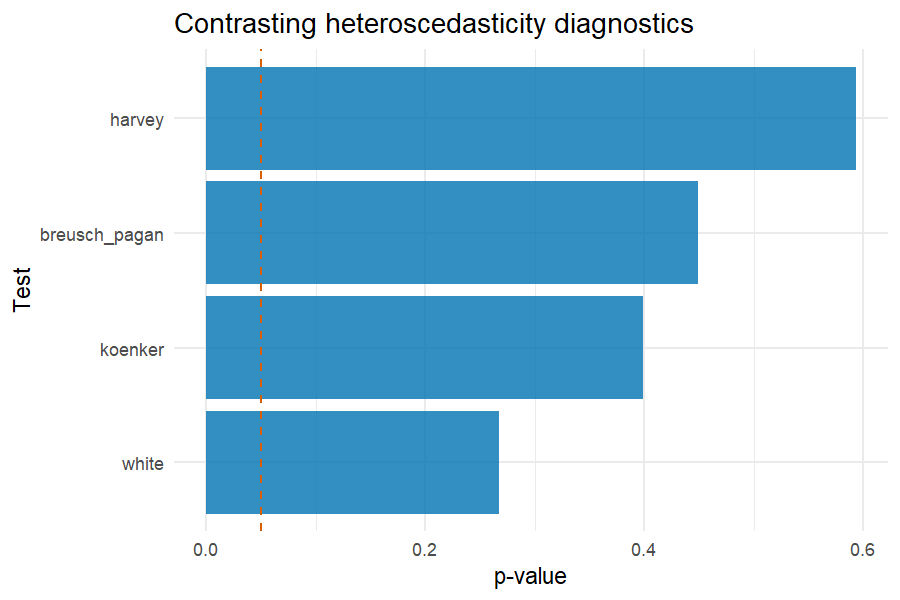
Interpretation. Koenker's robust variant is conservative in this moderate sample, whereas White's omnibus test remains sensitive to nonlinear variance. The RESET test also signals functional-form misspecification, suggesting that a variance stabilising transformation or spline terms could stabilise the error variance while addressing nonlinearity.

Summary

Across the three scenarios, heteroTests streamlines workflows by combining statistical theory with practical diagnostics. The package encourages analysts to inspect residual plots alongside formal tests and to validate remedies such as weighted least squares or variance modelling.